Numerical Analysis Chapter 3 Interpolation method Section 1

Numerical Analysis 上页 下页 返回

Chapter 3 Interpolation method Section 1 Introduction Section 2 Lagrange interpolation Section 3 Deviation and Newton interpolation Section 4 Difference and Equidistant interpolation Section 5 Hermite interpolation Section 6 Piecewise low-order interpolation Section 7 Cubic spline interpolation 上页 下页 返回

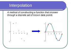
§ 1 Introduction The interpolation method is an important numerical method is widely used in theoretical research and engineering practice. The definition of interpolation method ： If function y = f (x) in the interval [a, b] are defined, and known the value of y 0, y 1 , … , yn is a ≤ x 0 < x 1< … < xn ≤ b, if having a simple function P(x), let P(xi ) = yi (i = 0, 1, …, n) is right，P(x) is called the interpolation function of f (x), spot x 0, x 1 , … , xn is called interpolation node , the interval [a, b] is called Interpolation interval, The method of solving interpolation 上页 function P(x) called interpolation method. 下页 返回

The geometric significance of interpolation method： Getting the solution of curve y = P (x) ，let it through given n+1 points (xi , yi )， i = 0, 1, …, n，and using it approximate the known curve y = f (x). 上页 下页 返回

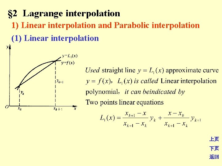
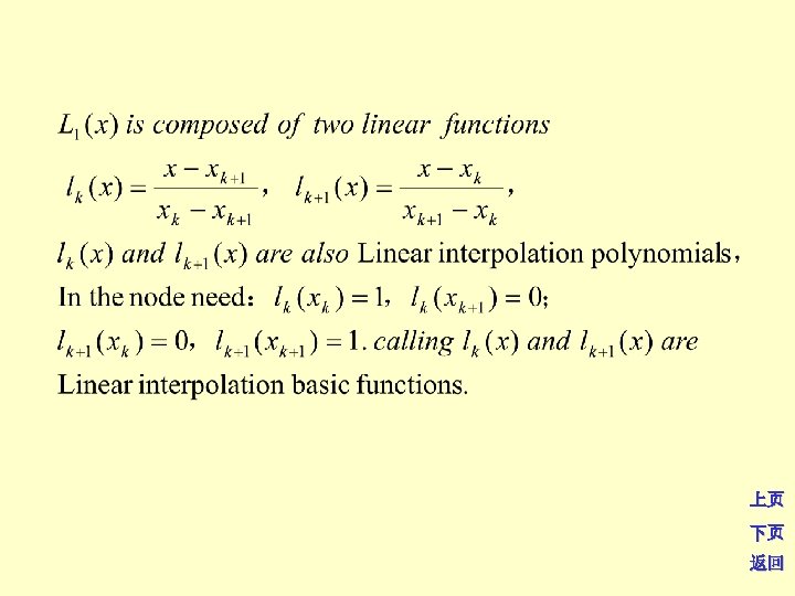
§ 2 Lagrange interpolation 1) Linear interpolation and Parabolic interpolation (1) Linear interpolation 上页 下页 返回

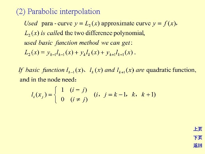
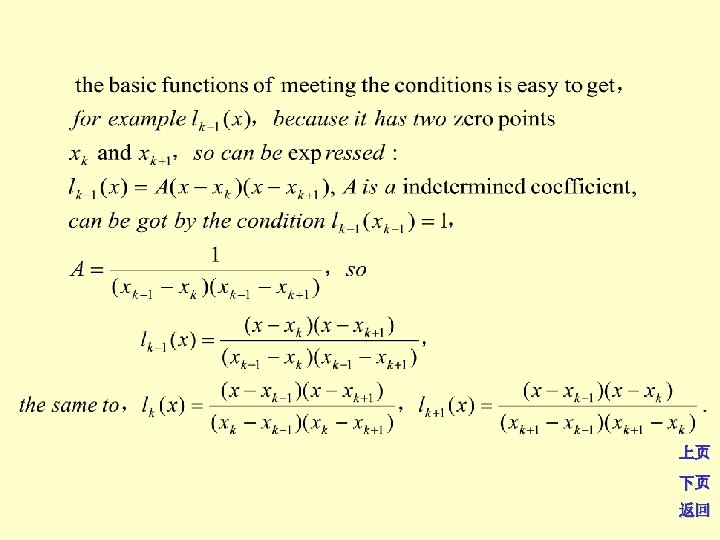
(2) Parabolic interpolation 上页 下页 返回

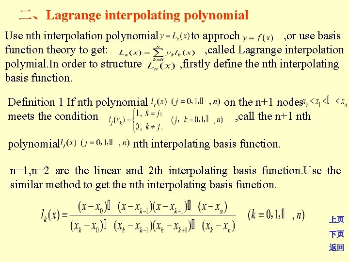
二、Lagrange interpolating polynomial Use nth interpolation polynomial function theory to get: polymial. In order to structure basis function. Definition 1 If nth polynomial meets the condition polynomial to approch , or use basis , called Lagrange interpolation , firstly define the nth interpolating on the n+1 nodes , call the n+1 nth interpolating basis function. n=1, n=2 are the linear and 2 th interpolating basis function. Use the similar method to get the nth interpolating basis function. 上页 下页 返回

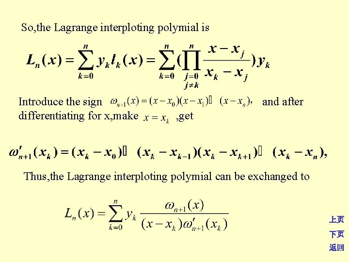
So, the Lagrange interploting polymial is Introduce the sign differentiating for x, make and after , get Thus, the Lagrange interploting polymial can be exchanged to 上页 下页 返回

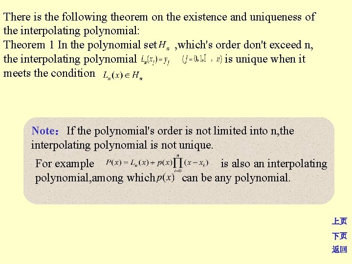
There is the following theorem on the existence and uniqueness of the interpolating polynomial: Theorem 1 In the polynomial set , which's order don't exceed n, the interpolating polynomial is unique when it meets the condition Note：If the polynomial's order is not limited into n, the interpolating polynomial is not unique. For example polynomial, among which is also an interpolating can be any polynomial. 上页 下页 返回

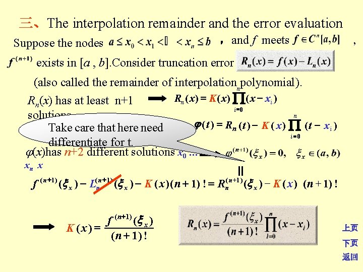
三、The interpolation remainder and the error evaluation ，and f meets , Suppose the nodes exists in [a , b]. Consider truncation error (also called the remainder of interpolationnpolynomial). Rn ( x) = K ( x) ( x xi ) Rn(x) has at least n+1 罗尔定理： 若 充分光滑， ，则 i =0 n solutions ( t ) = Rn ( t ) K ( x ) ( t x i ) 存在 使得 。 fixed x x i (i = 0, …, n), consider Take care that here need i=0 推广：若 differentiate for t. (x)has n+2 different solutions x 0 … 使得 使得 x x n f (n +1) (x x ) L(nn +1) (x x ) K ( x )( n + 1) ! = Rn( n 1 ) (x x ) K ( x ) ( n + 1) ! + 存在 使得 f ( n 1) (x x ) K ( x) = ( n + 1) ! + 上页 下页 返回

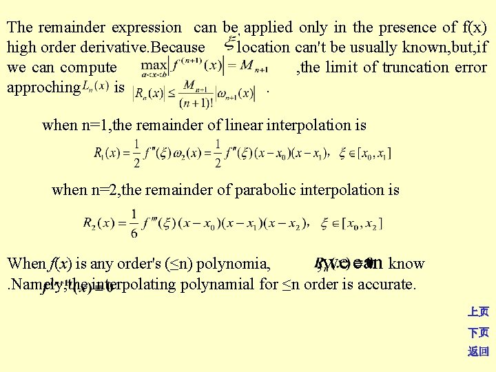
The remainder expression can be applied only in the presence of f(x) high order derivative. Because location can't be usually known, but, if we can compute , the limit of truncation error approching is. when n=1, the remainder of linear interpolation is when n=2, the remainder of parabolic interpolation is When f(x) is any order's (≤n) polynomia, , we can know. Namely, the interpolating polynamial for ≤n order is accurate. 上页 下页 返回

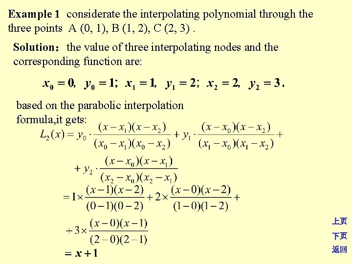
Example 1 considerate the interpolating polynomial through the three points A (0, 1), B (1, 2), C (2, 3). Solution：the value of three interpolating nodes and the corresponding function are: based on the parabolic interpolation formula, it gets: 上页 下页 返回

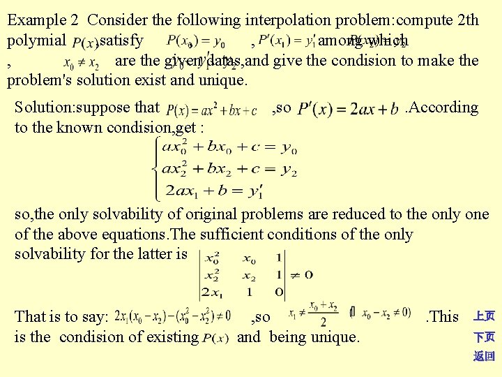
Example 2 Consider the following interpolation problem: compute 2 th polymial , satisfy , , among which , are the given datas, and give the condision to make the problem's solution exist and unique. Solution: suppose that to the known condision, get : , so . According so, the only solvability of original problems are reduced to the only one of the above equations. The sufficient conditions of the only solvability for the latter is That is to say: is the condision of existing , so and being unique. . This 上页 下页 返回

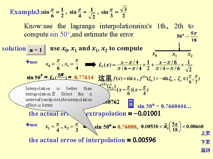
Example 3： Know: use the lagrange interpolationsinx's 1 th、 2 th to compute sin 50 , and estimate the error solution： n = 1 use x 0, x 1 and x 1, x 2 to compute use p sin 50 0 L 1 ( 5 ) 0. 77614 18 Interpolation is better than 而 extrapolation. If Select the x interval's endpoint, the interpolation effect is better. 这里 sin 50 = 0. 7660444… the actual error of extrapolation 0. 01001 use sin 50 0. 76008, the actual erroe of interpolation 0. 00596 上页 下页 返回

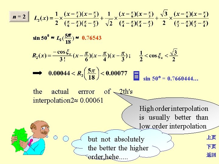
n = 2 p sin 50 0 L 2 ( 5 ) 0. 76543 18 the actual errror of interpolation 2 0. 00061 sin 50 = 0. 7660444… 2 th's High order interpolation is usually better than low order interpolation but not absolutely the better the higher order, hehe. . . 上页 下页 返回

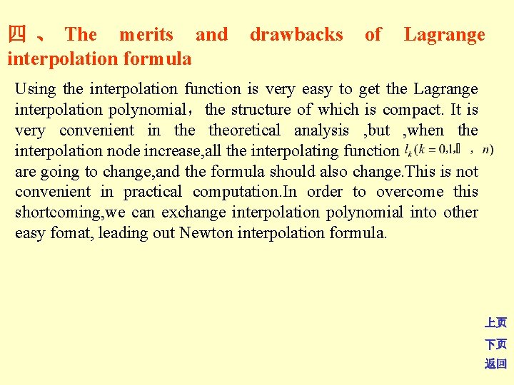
四 、 The merits and drawbacks of Lagrange interpolation formula Using the interpolation function is very easy to get the Lagrange interpolation polynomial，the structure of which is compact. It is very convenient in theoretical analysis , but , when the interpolation node increase, all the interpolating function are going to change, and the formula should also change. This is not convenient in practical computation. In order to overcome this shortcoming, we can exchange interpolation polynomial into other easy fomat, leading out Newton interpolation formula. 上页 下页 返回

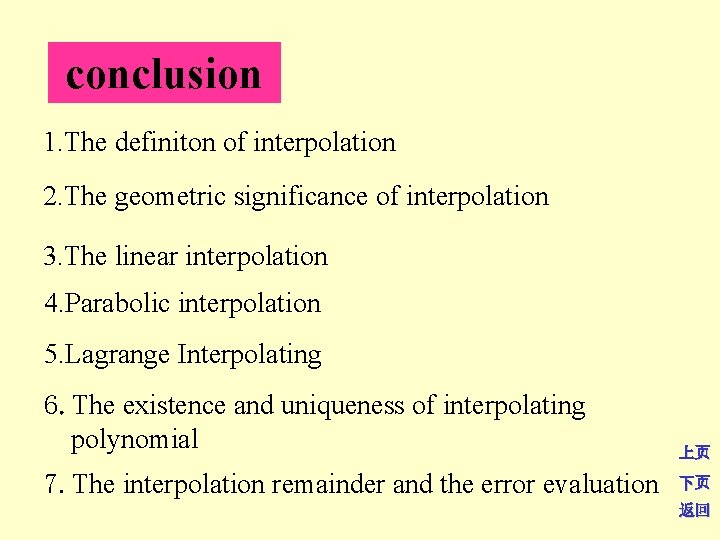
conclusion 1. The definiton of interpolation 2. The geometric significance of interpolation 3. The linear interpolation 4. Parabolic interpolation 5. Lagrange Interpolating 6. The existence and uniqueness of interpolating polynomial 7. The interpolation remainder and the error evaluation 上页 下页 返回

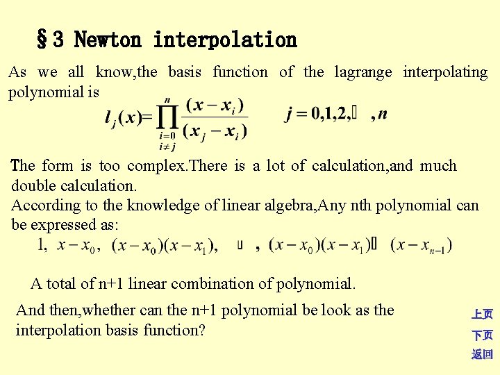
§ 3 Newton interpolation As we all know, the basis function of the lagrange interpolating polynomial is The form is too complex. There is a lot of calculation, and much double calculation. According to the knowledge of linear algebra, Any nth polynomial can be expressed as: A total of n+1 linear combination of polynomial. And then, whether can the n+1 polynomial be look as the interpolation basis function? 上页 下页 返回

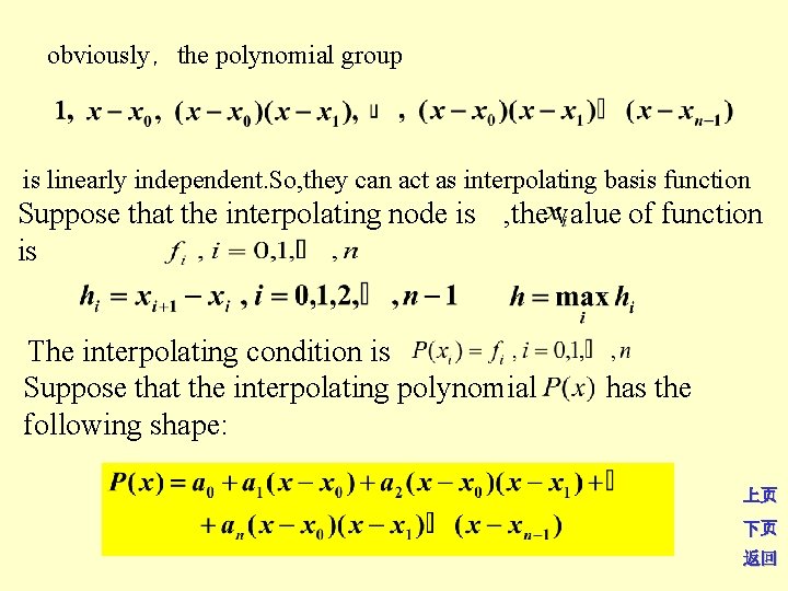
obviously，the polynomial group is linearly independent. So, they can act as interpolating basis function Suppose that the interpolating node is , the value of function is The interpolating condition is Suppose that the interpolating polynomial following shape: has the 上页 下页 返回

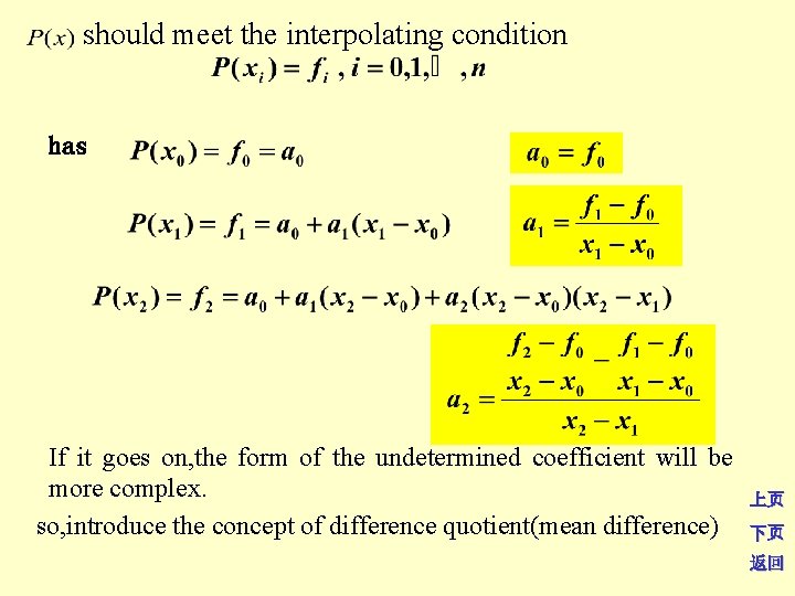
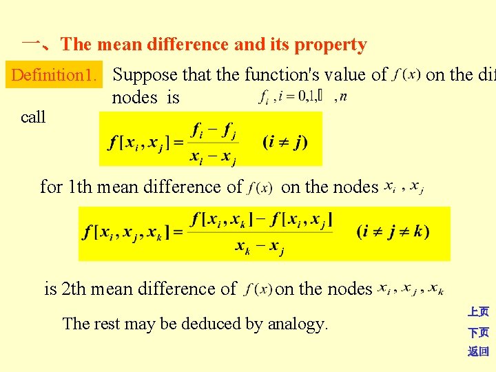
should meet the interpolating condition has If it goes on, the form of the undetermined coefficient will be more complex. so, introduce the concept of difference quotient(mean difference) 上页 下页 返回

一、The mean difference and its property Definition 1. Suppose that the function's value of call on the dif nodes is for 1 th mean difference of is 2 th mean difference of on the nodes The rest may be deduced by analogy. 上页 下页 返回

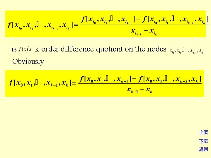
is k order difference quotient on the nodes Obviously 上页 下页 返回

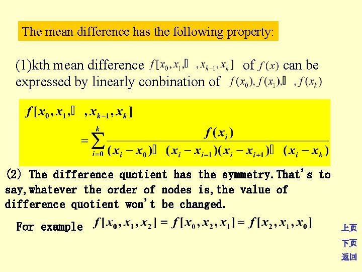
The mean difference has the following property: (1)kth mean difference expressed by linearly conbination of of can be (2) The difference quotient has the symmetry. That's to say, whatever the order of nodes is, the value of difference quotient won't be changed. For example 上页 下页 返回

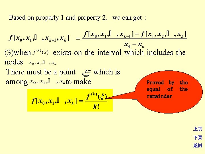
Based on property 1 and property 2，we can get： (3)when exists on the interval which includes the nodes There must be a point which is among to make Proved by the equal of remainder the 上页 下页 返回

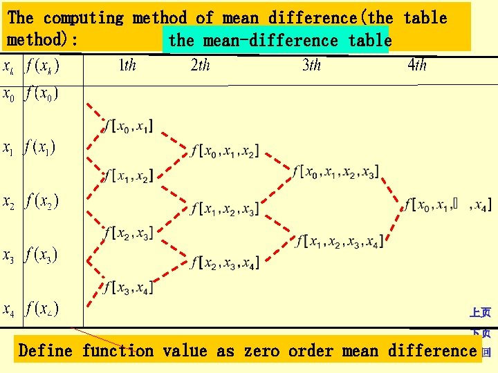
The computing method of mean difference(the table method): the mean-difference table 上页 下页 Define function value as zero order mean difference返回

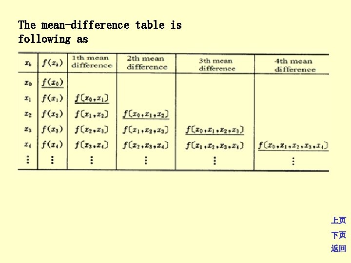
The mean-difference table is following as 上页 下页 返回

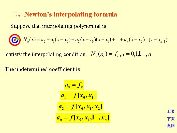
二、Newton’s interpolating formula Suppose that interpolating polynomial is satisfy the interpolating condition The undetermined coefficient is 上页 下页 返回

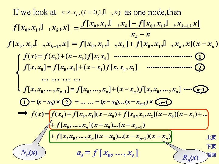
If we look at as one node, then 1 2 … … n 1 1 + (x x 0) 2 + … … + (x x 0)…(x xn 1) n 1 上页 Nn(x) ai = f [ x 0, …, xi ] 下页 Rn(x) 返回

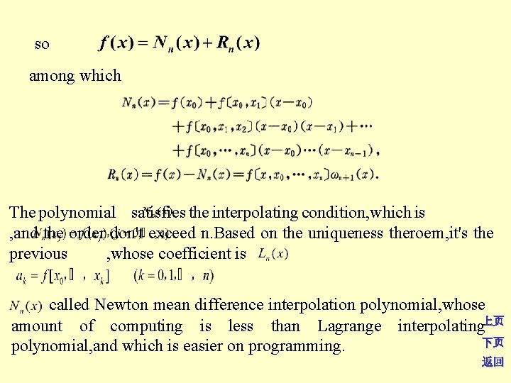
so among which The polynomial satisfies the interpolating condition, which is , and the order don't exceed n. Based on the uniqueness theroem, it's the previous , whose coefficient is called Newton mean difference interpolation polynomial, whose amount of computing is less than Lagrange interpolating上页 下页 polynomial, and which is easier on programming. 返回

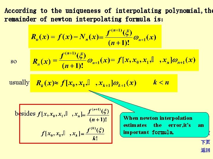
According to the uniqueness of interpolating polynomial, the remainder of newton interpolating formula is： so usually besides When newton interpolation estimates the error, it's an important formula. 上页 下页 返回

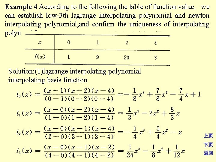
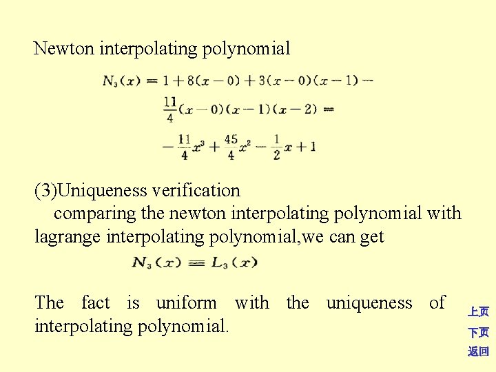
Example 4 According to the following the table of function value，we can establish low-3 th lagrange interpolating polynomial and newton interpolating polynomial, and confirm the uniqueness of interpolating polynomial. Solution: (1)lagrange interpolating polynomial interpolating basis function 上页 下页 返回

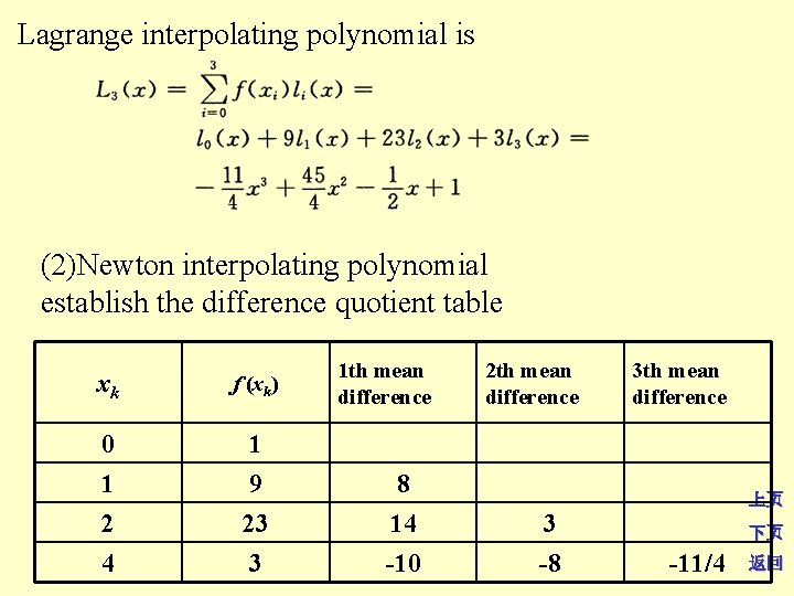
Lagrange interpolating polynomial is (2)Newton interpolating polynomial establish the difference quotient table 1 th mean difference xk f (xk) 0 1 1 9 8 2 4 23 3 14 -10 2 th mean difference 3 -8 3 th mean difference 上页 下页 -11/4 返回

Newton interpolating polynomial (3)Uniqueness verification comparing the newton interpolating polynomial with lagrange interpolating polynomial, we can get The fact is uniform with the uniqueness of interpolating polynomial. 上页 下页 返回

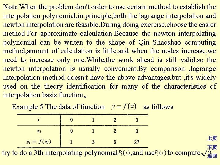
Note When the problem don't order to use certain method to establish the interpolation polynomial, in principle, both the lagrange interpolation and newton interpolation are feasible. During doing exercise, choose the easier method. For approximate calculation. Because the newton interpolating polynomial can be writen to the shape of Qin Shaoshao computing method, amount of calculation is little, and when the nodes increase, we need to increase only one. While, the work ahead is still valid. so the newton interpolation is usually convenient. By comparison , lagrange interpolation method doesn't have the above advantages, but , it's widely used on theory identification for many of the characteristics of interpolation basis function。 Example 5 The data of function as follows 上页 try to do a 3 th interpolating polynomial , and use to compute 下页 返回

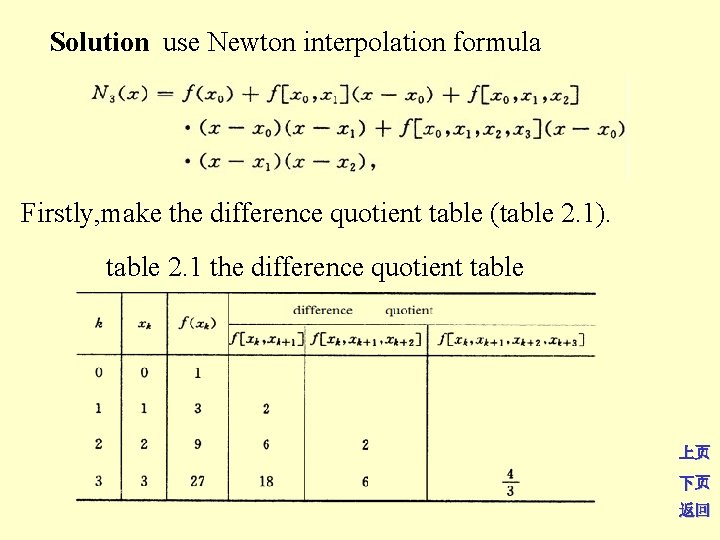
Solution use Newton interpolation formula Firstly, make the difference quotient table (table 2. 1). table 2. 1 the difference quotient table 上页 下页 返回

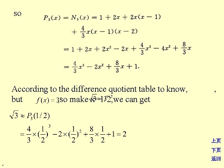
so According to the difference quotient table to know, but , so make x=1/2, we can get ， 上页 下页 返回 <

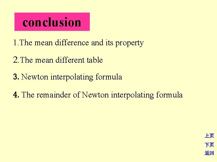
conclusion 1. The mean difference and its property 2. The mean different table 3. Newton interpolating formula 4. The remainder of Newton interpolating formula 上页 下页 返回

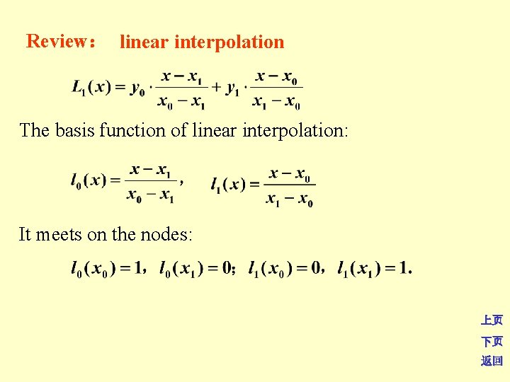
Review： linear interpolation The basis function of linear interpolation: It meets on the nodes: 上页 下页 返回

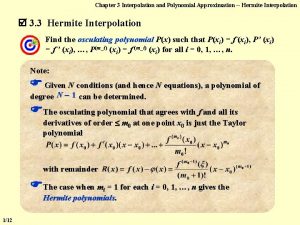
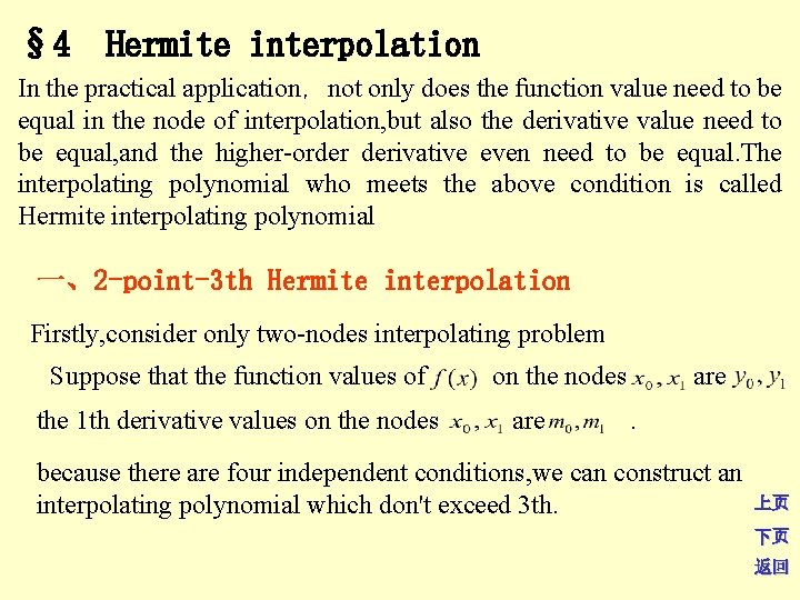
§ 4 Hermite interpolation In the practical application，not only does the function value need to be equal in the node of interpolation, but also the derivative value need to be equal, and the higher-order derivative even need to be equal. The interpolating polynomial who meets the above condition is called Hermite interpolating polynomial 一、2 -point-3 th Hermite interpolation Firstly, consider only two-nodes interpolating problem Suppose that the function values of the 1 th derivative values on the nodes are . because there are four independent conditions, we can construct an interpolating polynomial which don't exceed 3 th. 上页 下页 返回

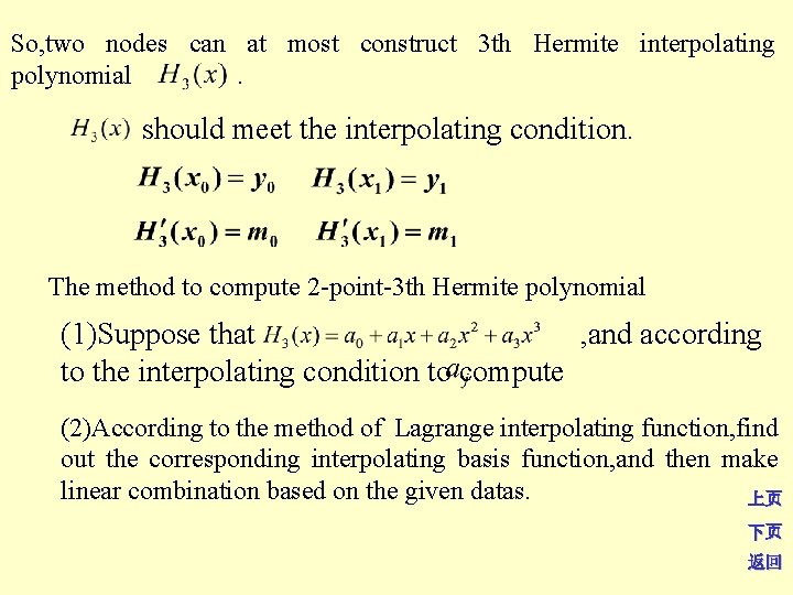
So, two nodes can at most construct 3 th Hermite interpolating polynomial. should meet the interpolating condition. The method to compute 2 -point-3 th Hermite polynomial (1)Suppose that , and according to the interpolating condition to compute (2)According to the method of Lagrange interpolating function, find out the corresponding interpolating basis function, and then make linear combination based on the given datas. 上页 下页 返回

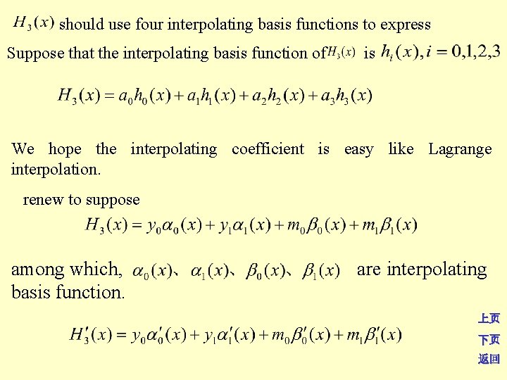
should use four interpolating basis functions to express Suppose that the interpolating basis function of is We hope the interpolating coefficient is easy like Lagrange interpolation. renew to suppose among which, basis function. are interpolating 上页 下页 返回

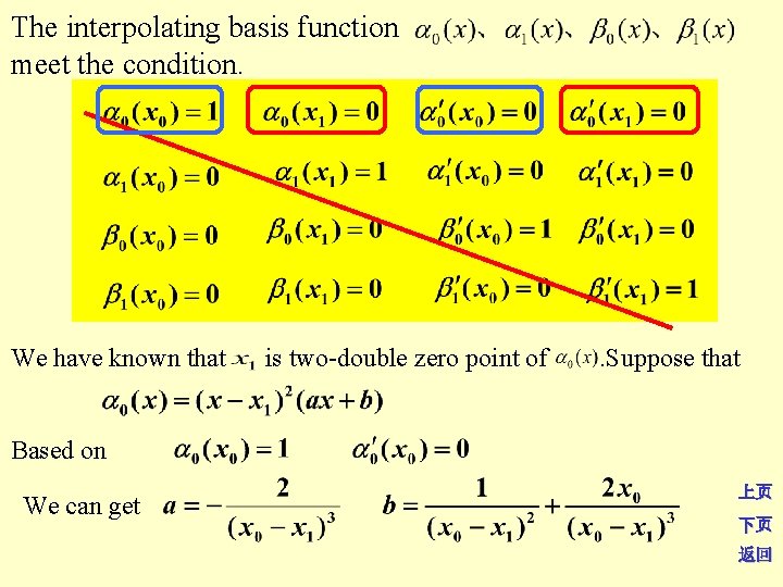
The interpolating basis function meet the condition. We have known that is two-double zero point of . Suppose that Based on We can get 上页 下页 返回

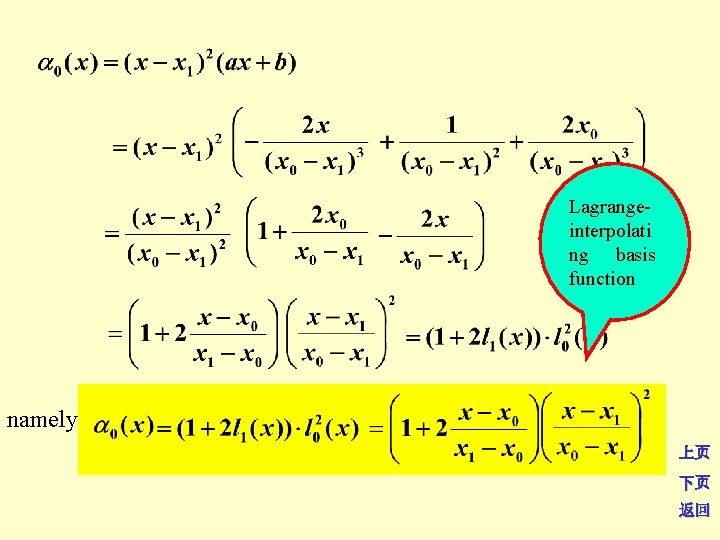
Lagrangeinterpolati ng basis function namely 上页 下页 返回

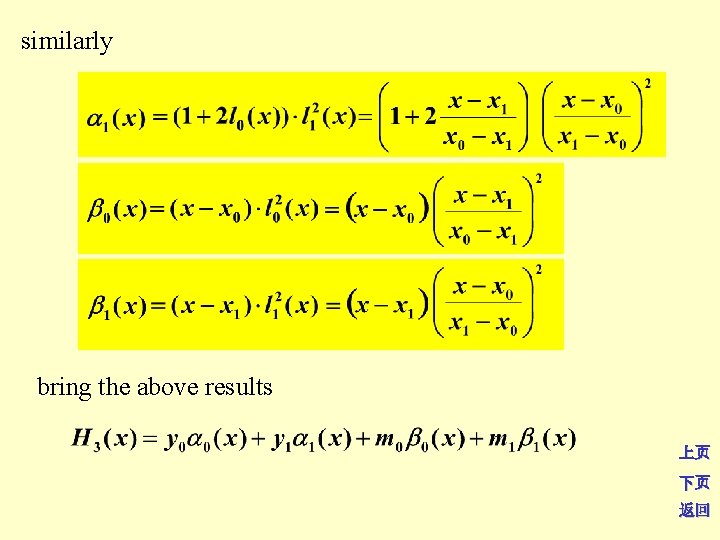
similarly bring the above results 上页 下页 返回

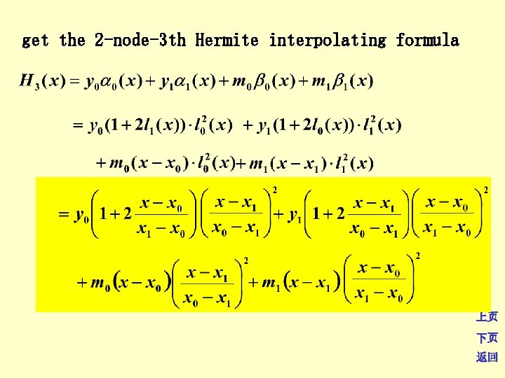
get the 2 -node-3 th Hermite interpolating formula 上页 下页 返回

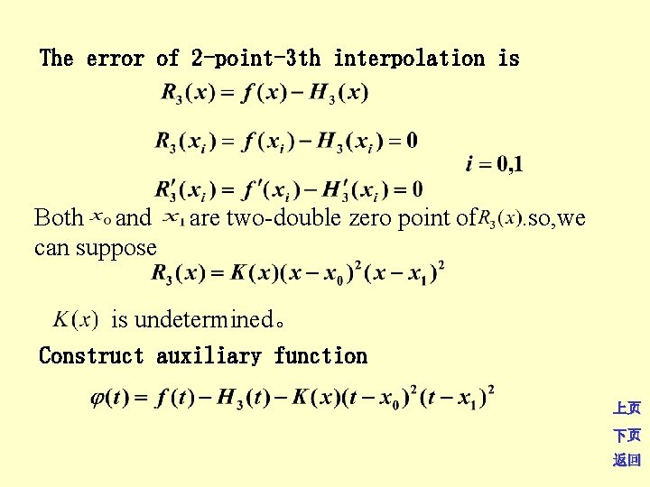
The error of 2 -point-3 th interpolation is Both and can suppose are two-double zero point of . so, we is undetermined。 Construct auxiliary function 上页 下页 返回

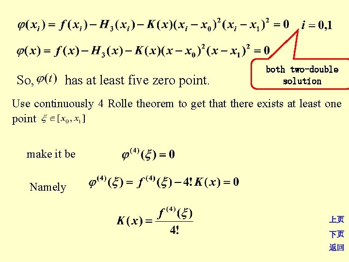
So, has at least five zero point. both two-double solution Use continuously 4 Rolle theorem to get that there exists at least one point make it be Namely 上页 下页 返回

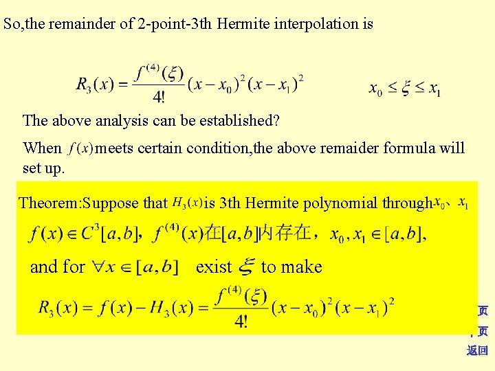
So, the remainder of 2 -point-3 th Hermite interpolation is The above analysis can be established? When set up. meets certain condition, the above remaider formula will Theorem: Suppose that and for is 3 th Hermite polynomial through exist to make 上页 下页 返回

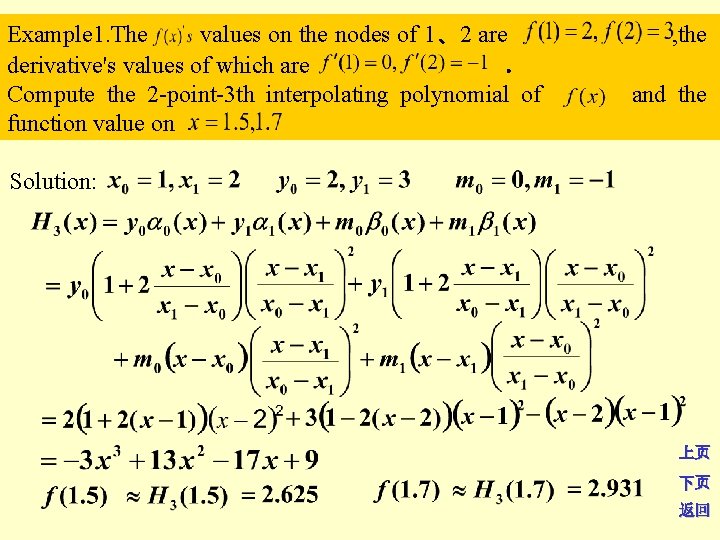
Example 1. The values on the nodes of 1、2 are derivative's values of which are. Compute the 2 -point-3 th interpolating polynomial of function value on , the and the Solution: 上页 下页 返回

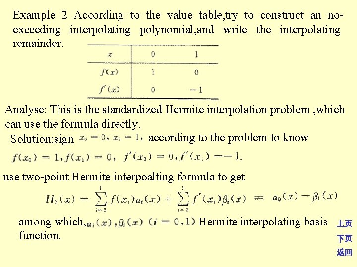
Example 2 According to the value table, try to construct an noexceeding interpolating polynomial, and write the interpolating remainder. Analyse: This is the standardized Hermite interpolation problem , which can use the formula directly. according to the problem to know Solution: sign use two-point Hermite interpoalting formula to get among which, function. is Hermite interpolating basis 上页 下页 返回

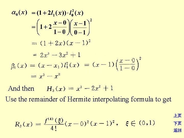
And then Use the remainder of Hermite interpolating formula to get 上页 下页 返回

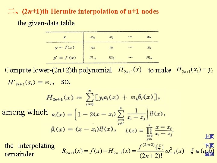
二、(2 n+1)th Hermite interpolation of n+1 nodes the given-data table Compute lower-(2 n+2)th polynomial to make so, among which 上页 the interpolating remainder 下页 返回

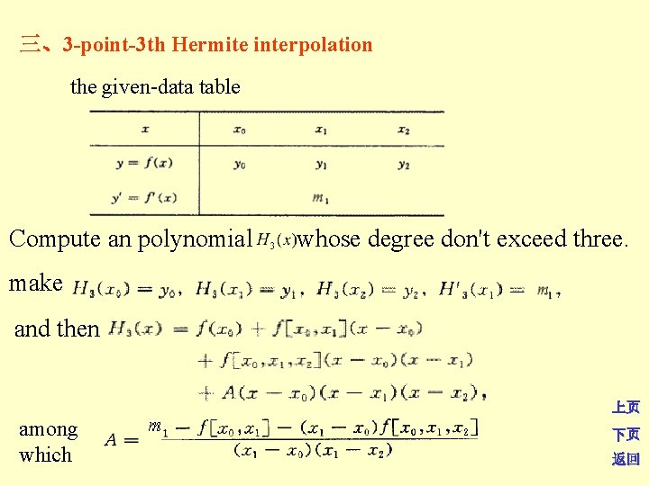
三、3 -point-3 th Hermite interpolation the given-data table Compute an polynomial whose degree don't exceed three. make and then 上页 among which 下页 返回

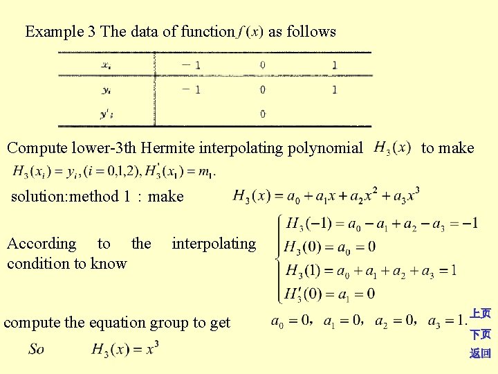
Example 3 The data of function as follows Compute lower-3 th Hermite interpolating polynomial to make solution: method 1：make According to the condition to know interpolating compute the equation group to get 上页 下页 返回

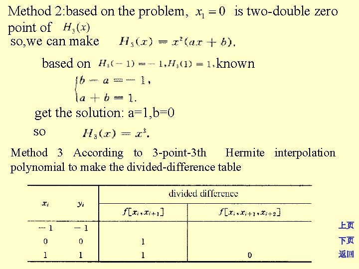
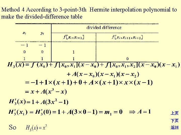
Method 2: based on the problem, point of so, we can make based on is two-double zero known get the solution: a=1, b=0 so Method 3 According to 3 -point-3 th Hermite interpolation polynomial to make the divided-difference table 上页 下页 返回

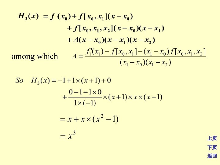
Method 4 According to 3 -point-3 th Hermite interpolation polynomial to make the divided-difference table 上页 下页 So 返回

conclusion 1. 2 -point-3 th Hermite interpolation 2. (2 n+1)th Hermite interpolation of n+1 nodes 3. 3 -point-3 th Hermite interpolation 上页 下页 返回

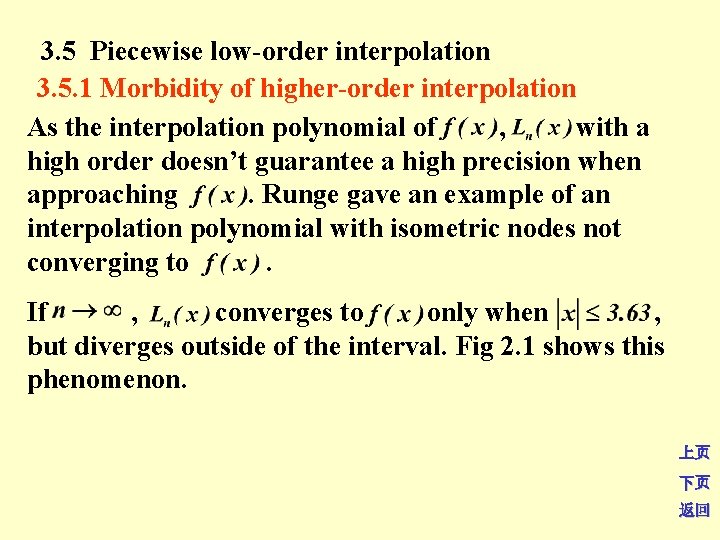
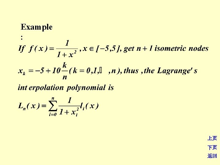
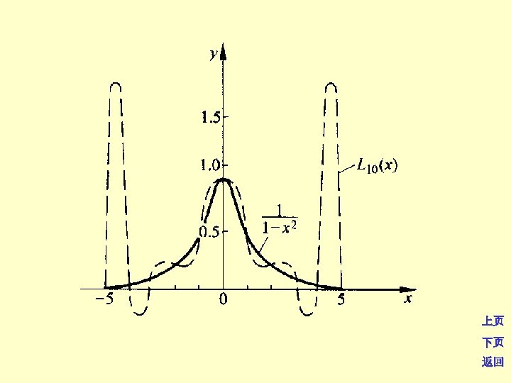
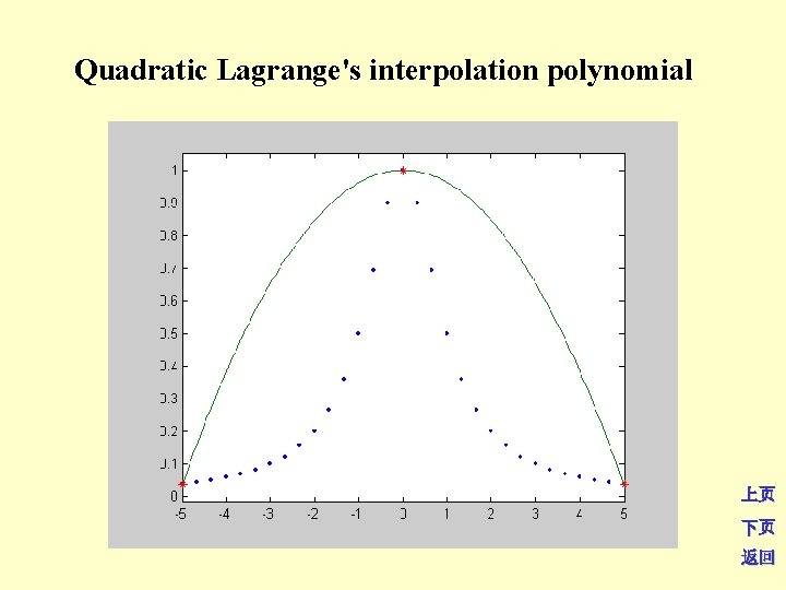
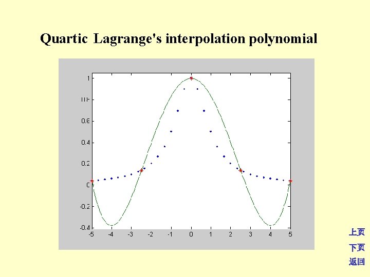
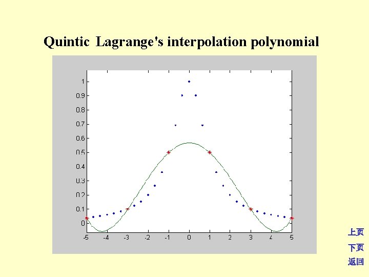
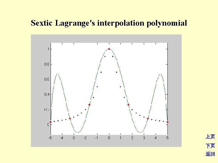
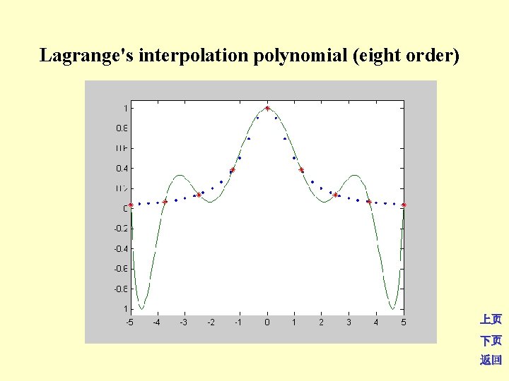
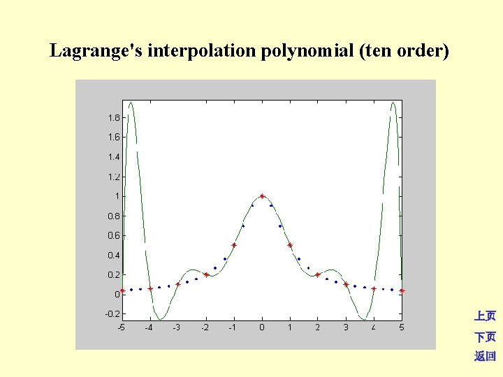
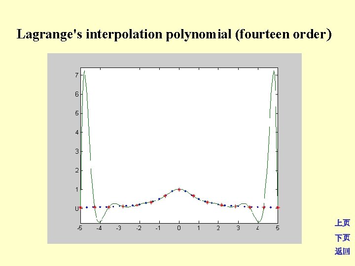
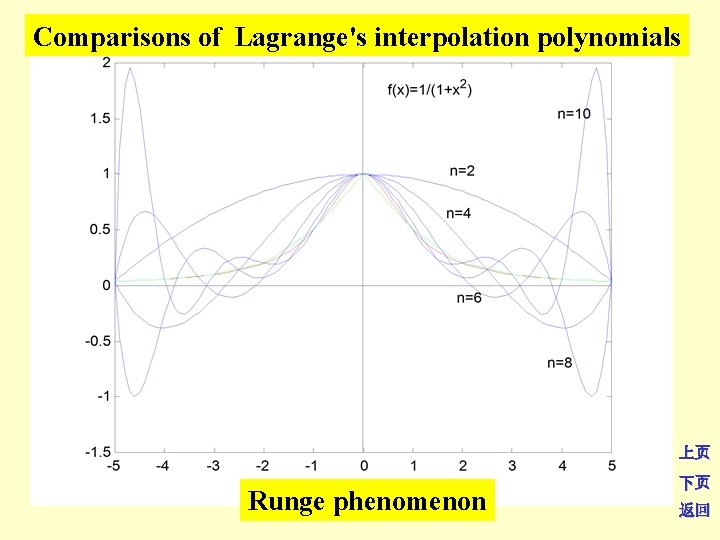
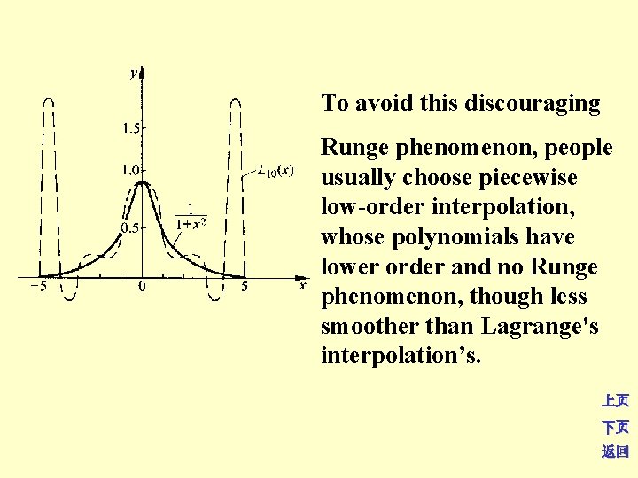
3. 5 Piecewise low-order interpolation 3. 5. 1 Morbidity of higher-order interpolation As the interpolation polynomial of , with a high order doesn’t guarantee a high precision when approaching . Runge gave an example of an interpolation polynomial with isometric nodes not converging to . If , converges to only when , but diverges outside of the interval. Fig 2. 1 shows this phenomenon. 上页 下页 返回

Quadratic Lagrange's interpolation polynomial 上页 下页 返回

Quartic Lagrange's interpolation polynomial 上页 下页 返回

Quintic Lagrange's interpolation polynomial 上页 下页 返回

Sextic Lagrange's interpolation polynomial 上页 下页 返回

Lagrange's interpolation polynomial (eight order) 上页 下页 返回

Lagrange's interpolation polynomial (ten order) 上页 下页 返回

Lagrange's interpolation polynomial (fourteen order) 上页 下页 返回

Comparisons of Lagrange's interpolation polynomials 上页 Runge phenomenon 下页 返回

To avoid this discouraging Runge phenomenon, people usually choose piecewise low-order interpolation, whose polynomials have lower order and no Runge phenomenon, though less smoother than Lagrange's interpolation’s. 上页 下页 返回

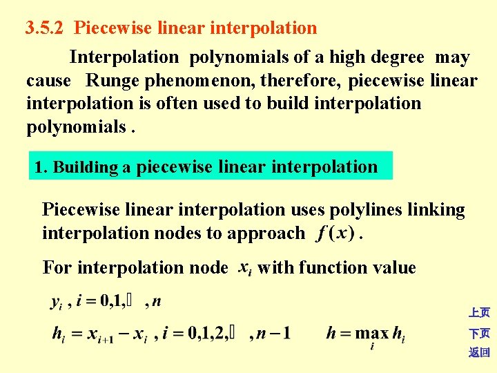
3. 5. 2 Piecewise linear interpolation Interpolation polynomials of a high degree may cause Runge phenomenon, therefore, piecewise linear interpolation is often used to build interpolation polynomials. 1. Building a piecewise linear interpolation Piecewise linear interpolation uses polylines linking interpolation nodes to approach . For interpolation node with function value 上页 下页 返回

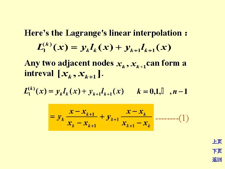
Here’s the Lagrange's linear interpolation ： Any two adjacent nodes can form a intreval . ----(1) 上页 下页 返回

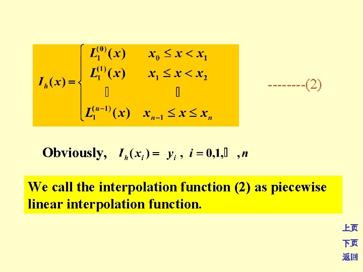
----(2) Obviously, We call the interpolation function (2) as piecewise linear interpolation function. 上页 下页 返回

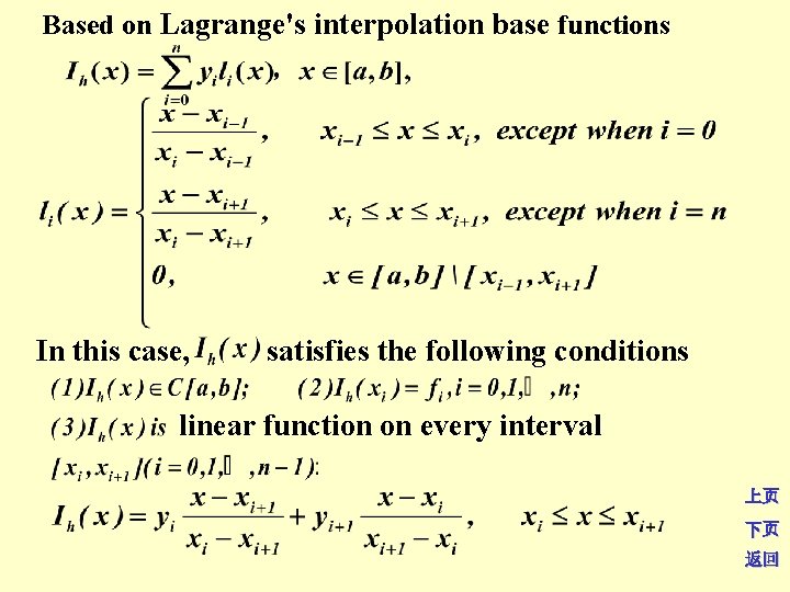
Based on Lagrange's interpolation base functions In this case, satisfies the following conditions linear function on every interval 上页 下页 返回

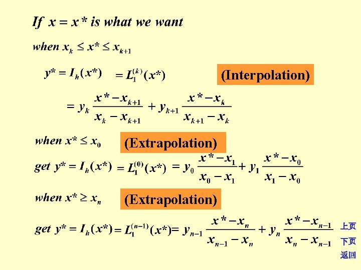
(Interpolation) (Extrapolation) 上页 下页 返回

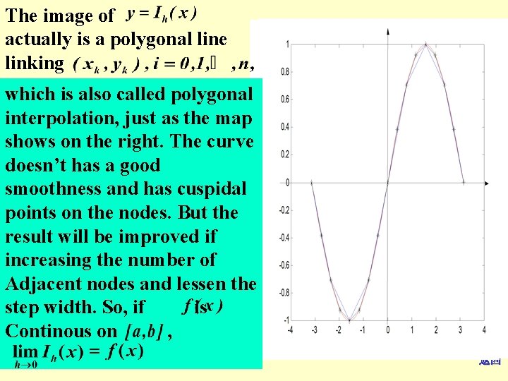
The image of actually is a polygonal line linking which is also called polygonal interpolation, just as the map shows on the right. The curve doesn’t has a good smoothness and has cuspidal points on the nodes. But the result will be improved if increasing the number of Adjacent nodes and lessen the step width. So, if is Continous on , 上页 下页 返回

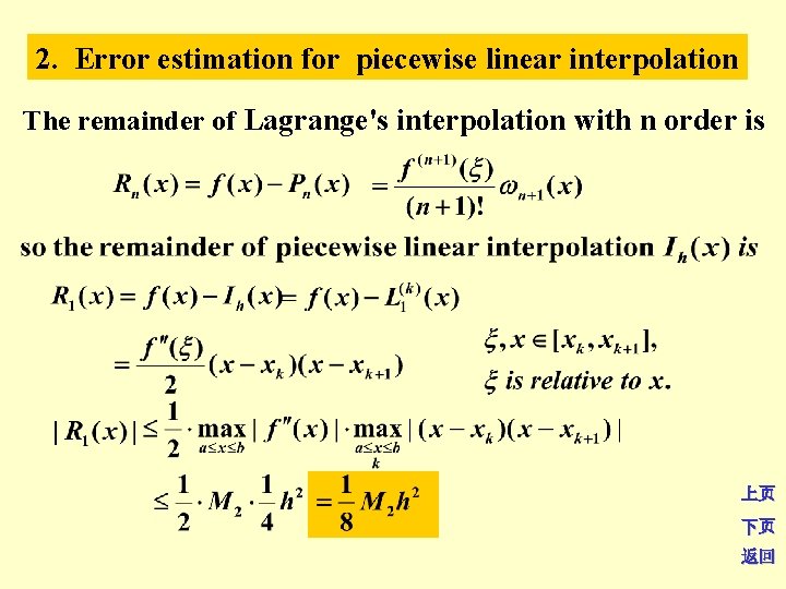
2. Error estimation for piecewise linear interpolation The remainder of Lagrange's interpolation with n order is 上页 下页 返回

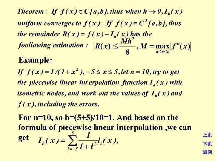
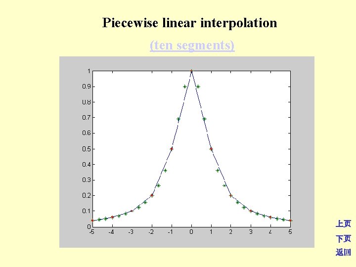
Example: For n=10, so h=(5+5)/10=1. And based on the formula of piecewise linear interpolation , we can get 上页 下页 返回

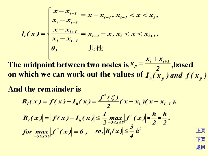
The midpoint between two nodes is , based on which we can work out the values of And the remainder is 上页 下页 返回

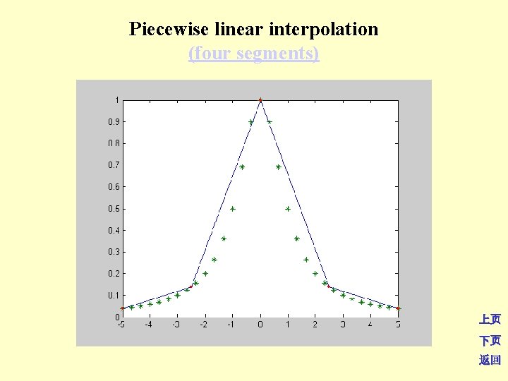
Piecewise linear interpolation (four segments) 上页 下页 返回

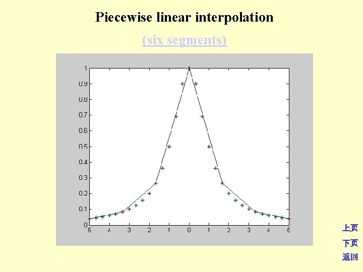
Piecewise linear interpolation (six segments) 上页 下页 返回

Piecewise linear interpolation (ten segments) 上页 下页 返回

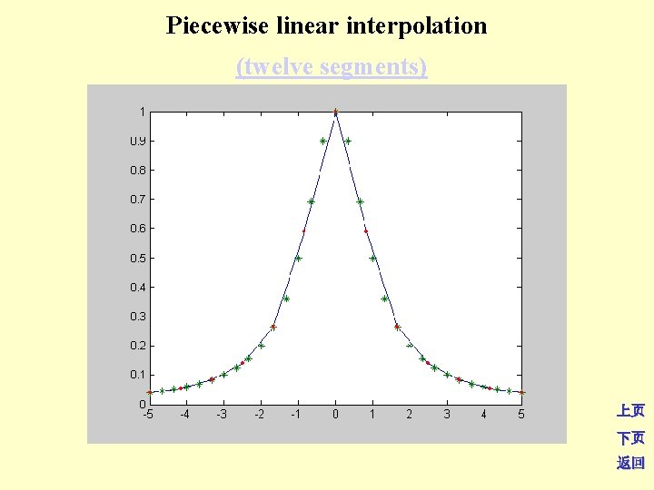
Piecewise linear interpolation (twelve segments) 上页 下页 返回

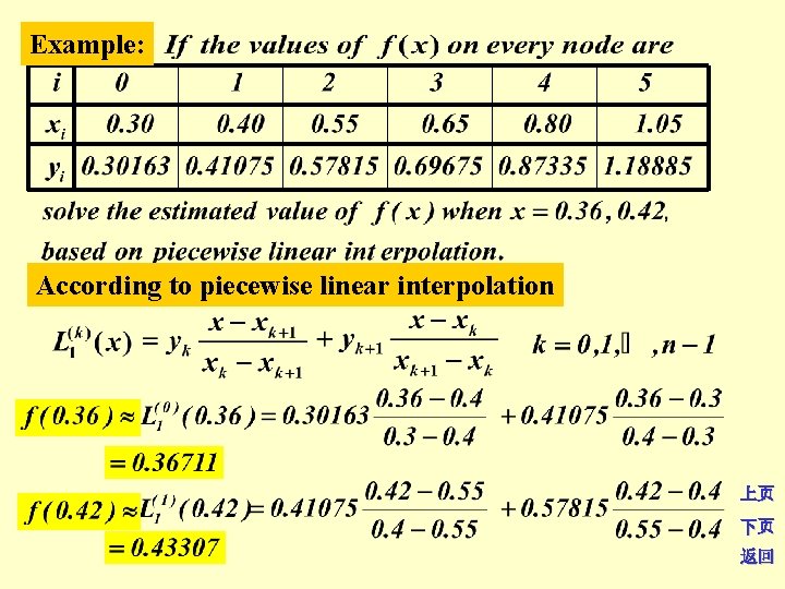
Example: According to piecewise linear interpolation 上页 下页 返回

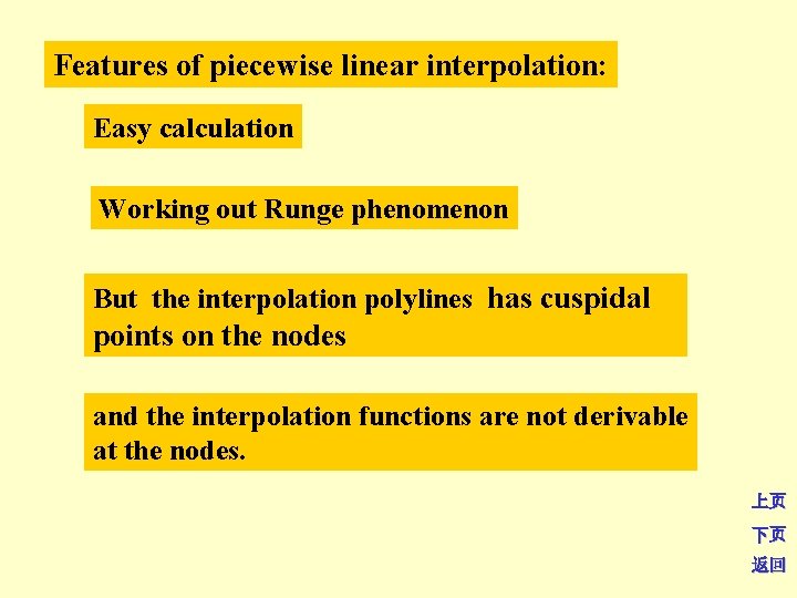
Features of piecewise linear interpolation: Easy calculation Working out Runge phenomenon But the interpolation polylines has cuspidal points on the nodes and the interpolation functions are not derivable at the nodes. 上页 下页 返回

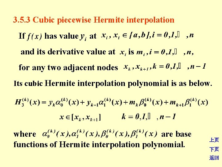
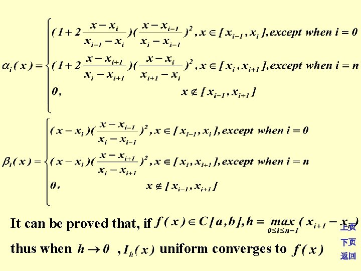
3. 5. 3 Cubic piecewise Hermite interpolation If has value at and its derivative value at is for any two adjacent nodes Its cubic Hermite interpolation polynomial is as below. where are base functions of Hermite interpolation polynomial. 上页 下页 返回

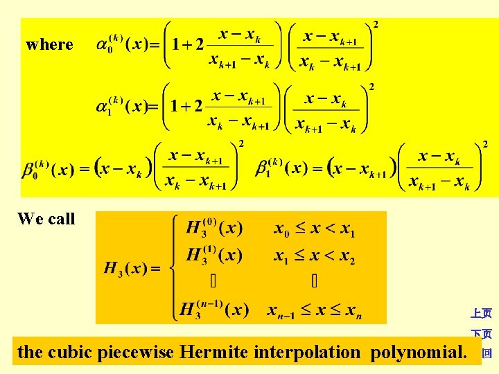
where We call 上页 下页 the cubic piecewise Hermite interpolation polynomial. 返回

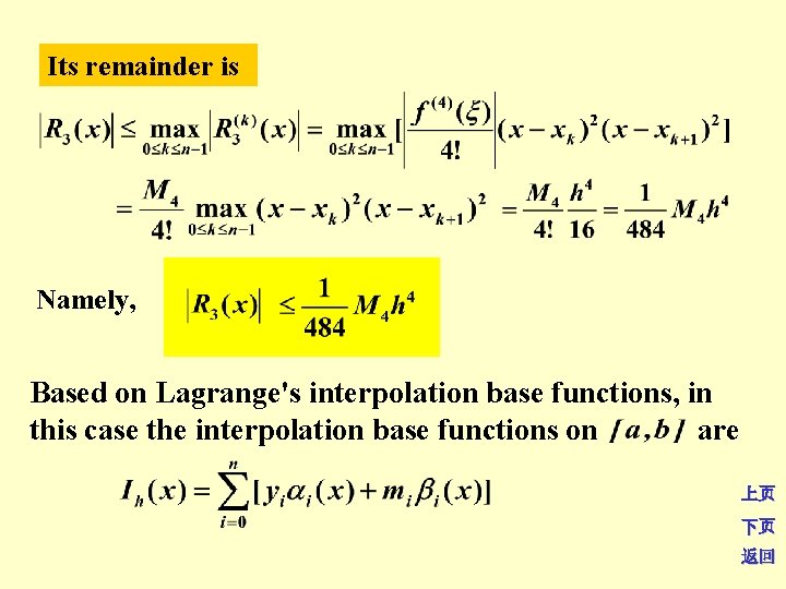
Its remainder is Namely, Based on Lagrange's interpolation base functions, in this case the interpolation base functions on are 上页 下页 返回

It can be proved that, if thus when , uniform converges to 上页 下页 返回

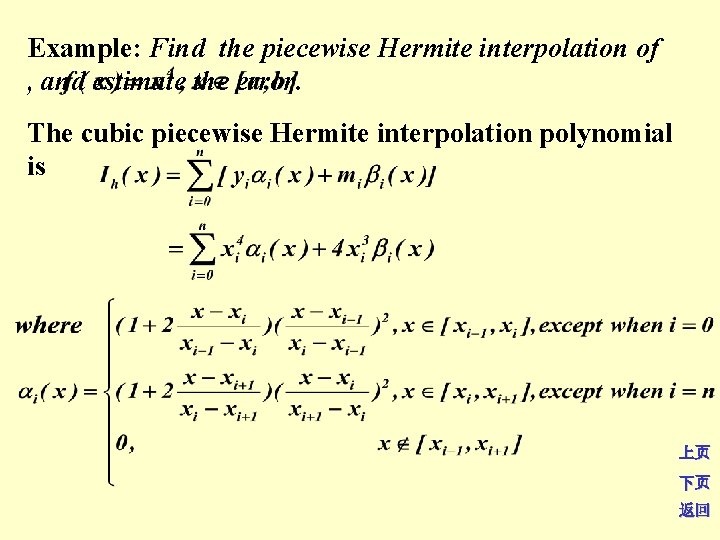
Example: Find the piecewise Hermite interpolation of , and estimate the error. The cubic piecewise Hermite interpolation polynomial is 上页 下页 返回

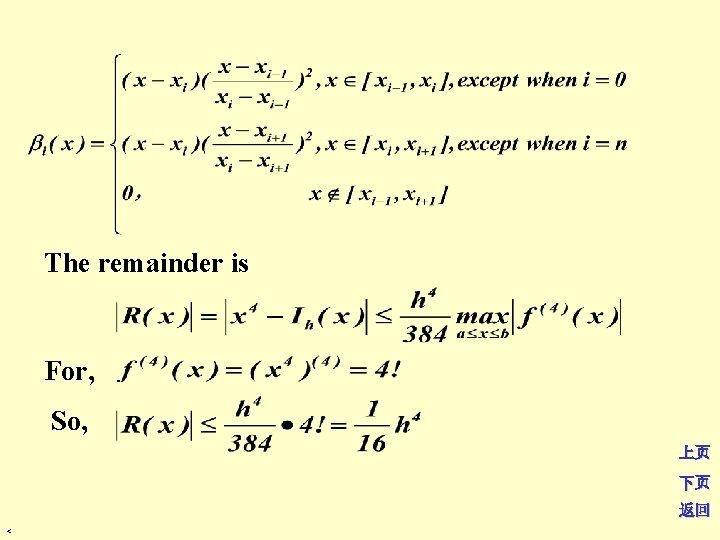
The remainder is For, So, 上页 下页 返回 <

Conclusion 1. Morbidity of higher-order interpolation 2. Piecewise linear Hermite interpolation 3. Cubic piecewise Hermite interpolation 上页 下页 返回

§ 6 cubic spline interpolation In the early aircraft and shipbuilding industry, Spline is the pin chip or metal wire which draughtsmen used to draw smooth curves. To get a smooth curve, they fasten the this procedure is called a spline function. spline to some adjacent points. Since the spline is flexible, it forms a smooth curve passing the points. At mathematics a function imitating Piecewise linear interpolation and piecewise Hermite interpolation functions are not smooth enough. Moreover, it’s difficult to get the derivation at the nodes. Spline interpolation is using piecewise low-order polynomials to approach functions. It satisfies the smoothness and doesn’t need the 上页 derivation at the nodes. All needed are the values at every 下页 node and the information of two frontier nodes’ derivation. 返回

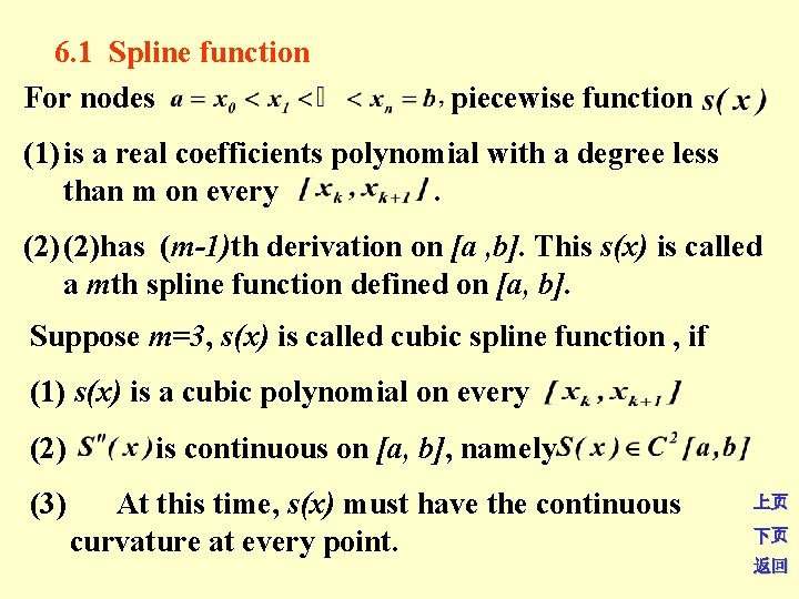
6. 1 Spline function For nodes piecewise function (1) is a real coefficients polynomial with a degree less than m on every . (2)has (m-1)th derivation on [a , b]. This s(x) is called a mth spline function defined on [a, b]. Suppose m=3, s(x) is called cubic spline function , if (1) s(x) is a cubic polynomial on every (2) is continuous on [a, b], namely (3) At this time, s(x) must have the continuous curvature at every point. 上页 下页 返回

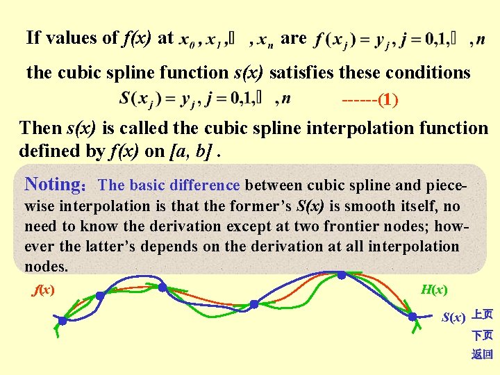
If values of f(x) at are the cubic spline function s(x) satisfies these conditions ------(1) Then s(x) is called the cubic spline interpolation function defined by f(x) on [a, b]. Noting：The basic difference between cubic spline and piecewise interpolation is that the former’s S(x) is smooth itself, no need to know the derivation except at two frontier nodes; however the latter’s depends on the derivation at all interpolation nodes. f(x) H(x) S(x) 上页 下页 返回

6. 2 Building a cubic spline interpolation function 1. Three angles rotating method Supposing a division of [a, b], f(x) has values at nodes If s(x) is the cubic spline interpolation function of f(x), then it must meets ------(2) 上页 下页 返回

S(x) has to meet above four groups (4 n-2) conditions S(x) is a piecewise function, namely ------(3) Sk(x) is a cubic spline polynomial defined on ------(4) 上页 下页 返回

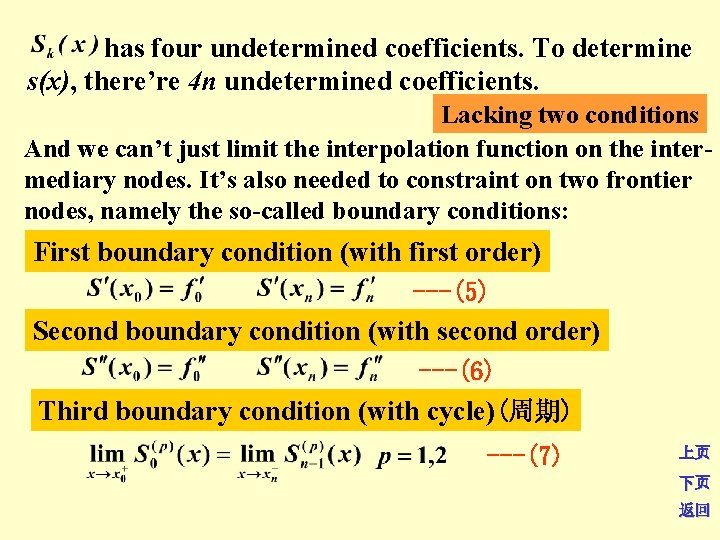
has four undetermined coefficients. To determine s(x), there’re 4 n undetermined coefficients. Lacking two conditions And we can’t just limit the interpolation function on the intermediary nodes. It’s also needed to constraint on two frontier nodes, namely the so-called boundary conditions: First boundary condition (with first order) ---(5) Second boundary condition (with second order) ---(6) Third boundary condition (with cycle)(周期) ---(7) 上页 下页 返回

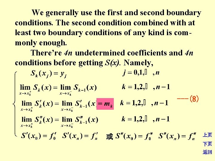
We generally use the first and second boundary conditions. The secondition combined with at least two boundary conditions of any kind is commonly enough. There’re 4 n undetermined coefficients and 4 n conditions before getting S(x). Namely, ---(8) 或 上页 下页 返回

Supposing ------(9) Then here’s the cubic interpolation polynomial of f(x) on , expressed in the form of cubic Hermite interpolation. 上页 下页 返回

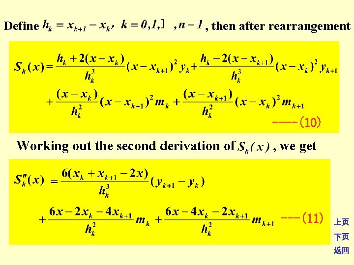
Define , then after rearrangement ----(10) Working out the second derivation of , we get ---(11) 上页 下页 返回

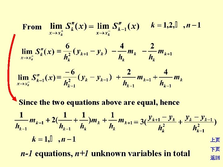
From Since the two equations above are equal, hence 上页 n-1 equations, n+1 unknown variables in total 下页 返回

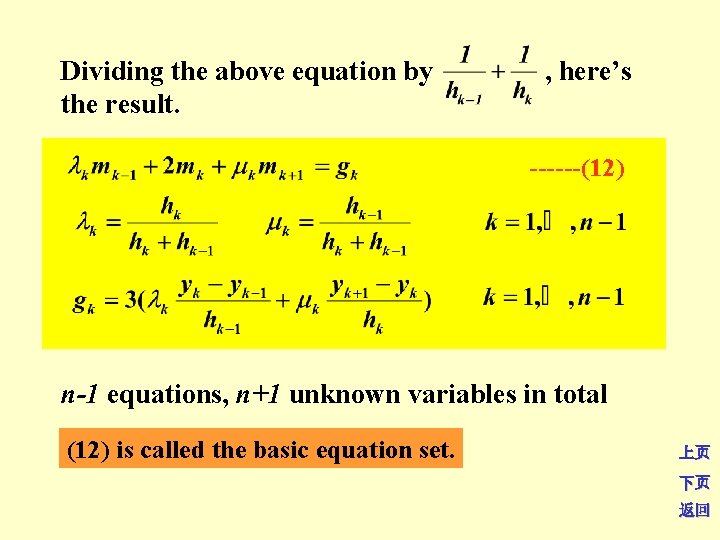
Dividing the above equation by , here’s the result. ------(12) n-1 equations, n+1 unknown variables in total (12) is called the basic equation set. 上页 下页 返回

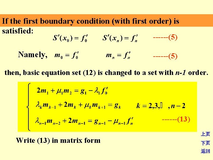
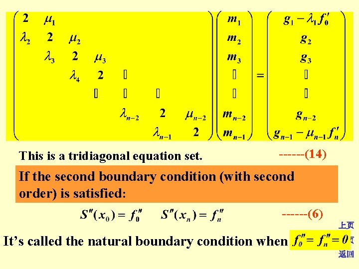
If the first boundary condition (with first order) is satisfied: ------(5) Namely, ------(5) then, basic equation set (12) is changed to a set with n-1 order. ------(13) Write (13) in matrix form 上页 下页 返回

This is a tridiagonal equation set. ------(14) If the second boundary condition (with second order) is satisfied: ------(6) 上页 It’s called the natural boundary condition when 下页 返回

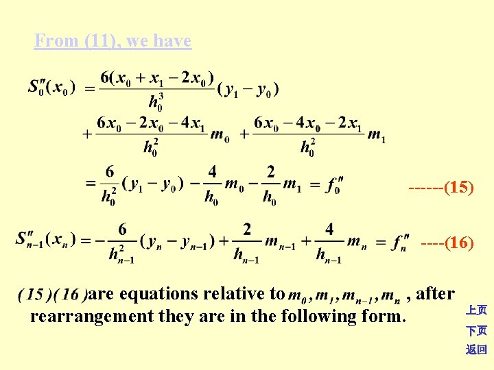
From (11), we have ------(15) ----(16) are equations relative to , after rearrangement they are in the following form. 上页 下页 返回

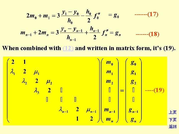
------(17) ------(18) When combined with (12) and written in matrix form, it’s (19). ----(19) 上页 下页 返回

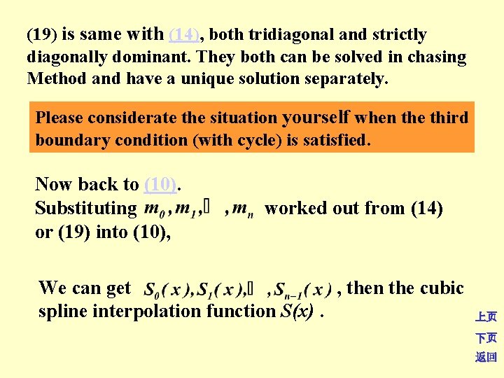
(19) is same with (14), both tridiagonal and strictly diagonally dominant. They both can be solved in chasing Method and have a unique solution separately. Please considerate the situation yourself when the third boundary condition (with cycle) is satisfied. Now back to (10). Substituting worked out from (14) or (19) into (10), We can get , then the cubic spline interpolation function S(x). 上页 下页 返回

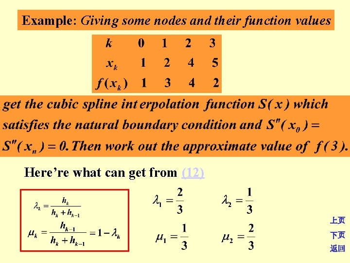
Example: Giving some nodes and their function values Here’re what can get from (12) 上页 下页 返回

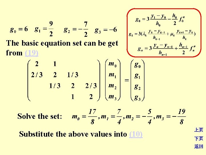
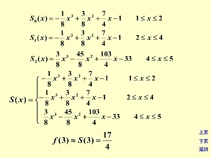
The basic equation set can be get from (19) Solve the set: Substitute the above values into (10) 上页 下页 返回

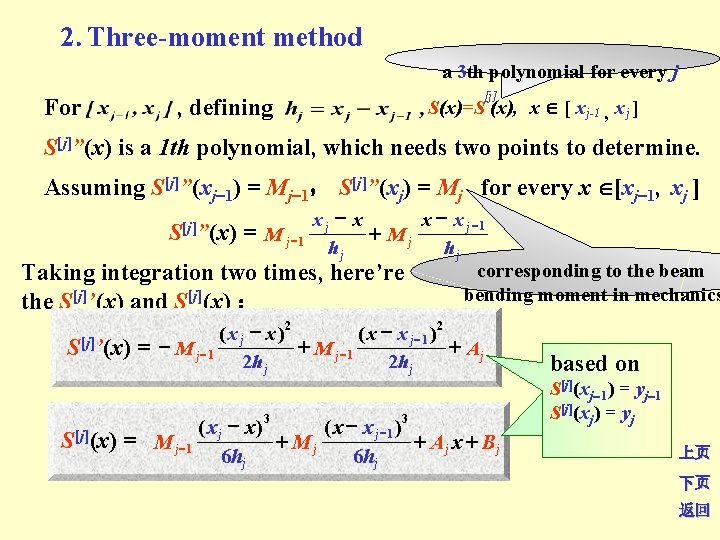
2. Three-moment method a 3 th polynomial for every j [j] S(x)=S (x), x [ x j-1 , x j ] For , defining S[j]”(x) is a 1 th polynomial, which needs two points to determine. Assuming S[j]”(xj 1) = Mj 1， S[j]”(xj) = Mj for every x [xj 1, xj ] xj x x x j 1 +Mj M j 1 hj hj corresponding to the beam Taking integration two times, here’re bending moment in mechanics the S[j]’(x) and S[j](x) ： S[j]”(x) = S[j]’(x) = ( x j x )2 ( x x j 1 ) 2 M j 1 + Aj 2 h j ( x j x) ( x x j 1 ) [j] + Mj + Aj x + B j S (x) = M j 1 6 hj 3 3 based on S[j](xj 1) = yj 1 S[j](xj) = yj 上页 下页 返回

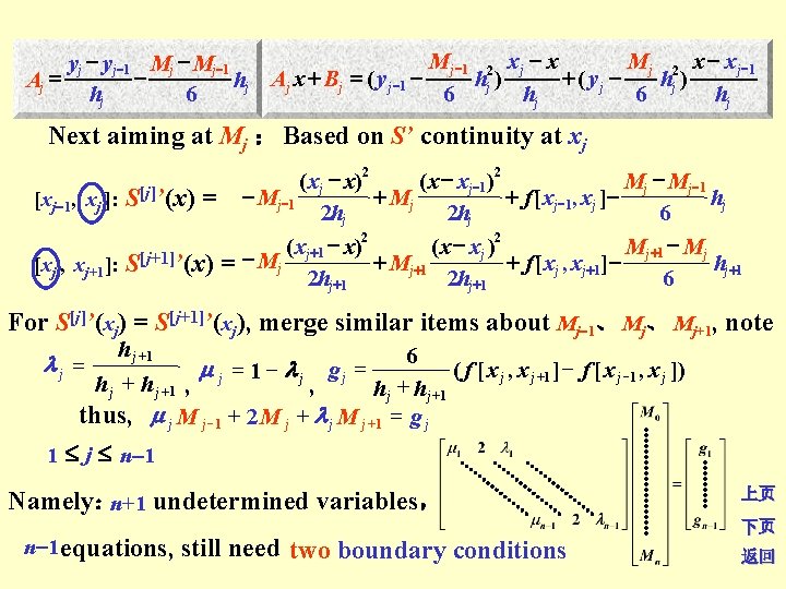
yj yj 1 Mj 1 Aj = hj hj 6 M j 1 2 x j x M j 2 x x j 1 + ( yj Aj x + Bj = ( y j 1 hj ) 6 hj Next aiming at Mj ： Based on S’ continuity at xj 2 2 ( x x ) Mj 1 j j 1 [j] + Mj + f [ xj 1 , xj ] hj [xj 1, xj ]: S ’(x) = Mj 1 2 hj 6 2 2 ( x x ) Mj+1 Mj + j 1 j [j+1] + Mj+1 + f [ xj , xj+1 ] hj+1 [xj , xj+1]: S ’(x) = Mj 2 hj+1 6 For S[j]’(xj) = S[j+1]’(xj), merge similar items about Mj 1、 Mj+1, note h j +1 6 j = 1 j gj = ( f [ x j , x j +1 ] f [ x j 1 , x j ]) h j +1 , h j +1 thus, j M j 1 + 2 M j + j M j +1 = g j 1 j n 1 Namely： undetermined variables， n+1 n 1 equations, still need two boundary conditions 上页 下页 返回

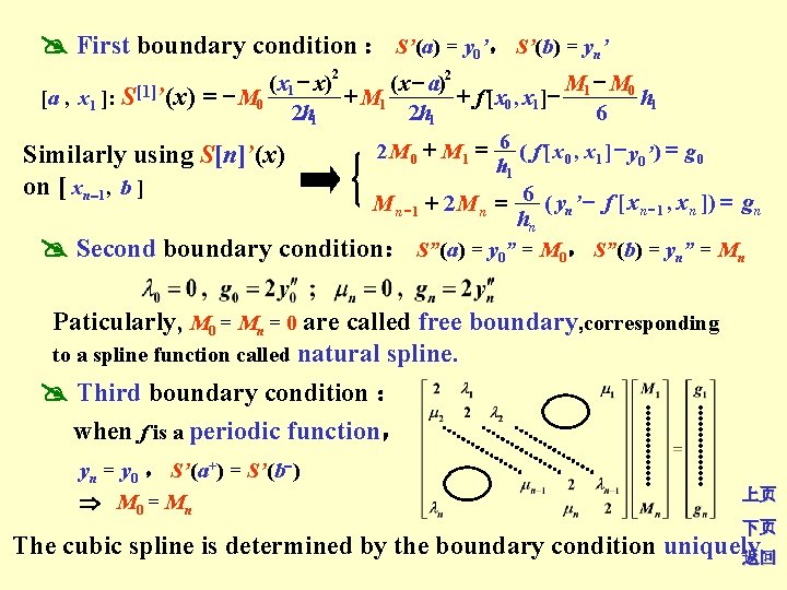
First boundary condition ： S’(a) = y 0’， S’(b) = yn’ 2 2 M M 0 ( x x ) ( x a ) 1 + M 1 + f [ x 0 , x 1 ] 1 [a , x 1 ]: S[1]’(x) = M 0 h 1 2 h 1 6 2 M 0 + M 1 = 6 ( f [ x 0 , x 1 ] y 0 ’ ) = g 0 Similarly using S[n]’(x) h 1 on [ xn 1, b ] M n 1 + 2 M n = 6 ( yn’ f [ x n 1 , x n ]) = g n hn Second boundary condition： S”(a) = y 0” = M 0， S”(b) = yn” = Mn Paticularly, M 0 = Mn = 0 are called free boundary, corresponding to a spline function called natural spline. Third boundary condition ： when f is a periodic function， yn = y 0 ， S’(a+) = S’(b ) M 0 = Mn 上页 下页 The cubic spline is determined by the boundary condition uniquely. 返回

At last, take a look at the convergence quality. Theorem: Assuming f(x)∈C 2[a, b], S(x) is a cubic spline interpolation function satisfying any boundary conditions taking xk (k=0, 1, …, n) as nodes. If when converge to And if thus, 上页 下页 返回

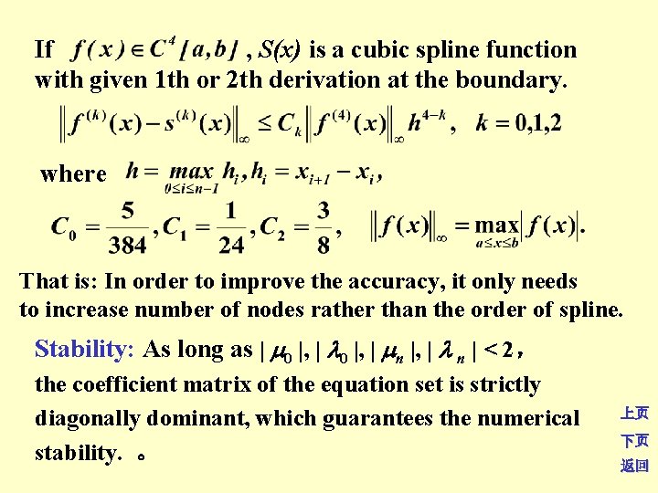
If , S(x) is a cubic spline function with given 1 th or 2 th derivation at the boundary. where That is: In order to improve the accuracy, it only needs to increase number of nodes rather than the order of spline. Stability: As long as | 0 |, | n |, | n | < 2， the coefficient matrix of the equation set is strictly diagonally dominant, which guarantees the numerical stability. 。 上页 下页 返回

conclusion 1. Spline function 2. Three angles rotating method to build cubic spline interpolation function 3. Three-moment method to build cubic spline interpolation function 上页 下页 返回

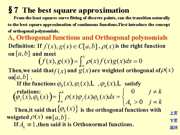
§ 7 The best square approximation From the least squares curve fitting of discrete points, can the transition naturally to the best square approximation of continuous functions. First introduce the concept of orthogonal polynomials. A, Orthogonal functions and Orthogonal polynomials Definition: If , is the right function on and meet Then, we said that and are weighted orthogonal of on . If the functions satisfy relations: Then, it said that is the orthogonal functions with weigeted on . If , then said it is Orthonormal functions. 上页 下页 返回

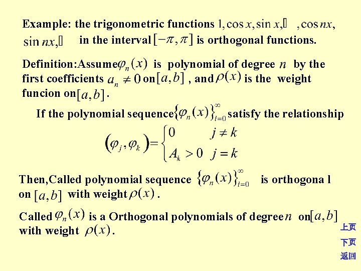
Example: the trigonometric functions in the interval is orthogonal functions. Definition: Assume is polynomial of degree by the first coefficients on , and is the weight funcion on . If the polynomial sequence satisfy the relationship Then, Called polynomial sequence is orthogona l on with weight . Called is a Orthogonal polynomials of degree on 上页 with weight . 下页 返回

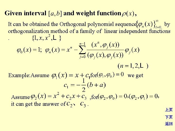
Given interval and weight function , It can be obtained the Orthogonal polynomisl sequence by orthogonalization method of a family of linear independent functions. Example: Assume it can get the answer of , for we get , for. 上页 下页 返回

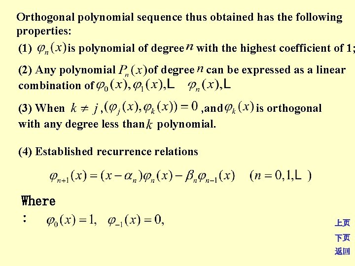
Orthogonal polynomial sequence thus obtained has the following properties: (1) is polynomial of degree with the highest coefficient of 1; (2) Any polynomial of degree can be expressed as a linear combination of (3) When , , and is orthogonal with any degree less than polynomial. (4) Established recurrence relations Where : 上页 下页 返回

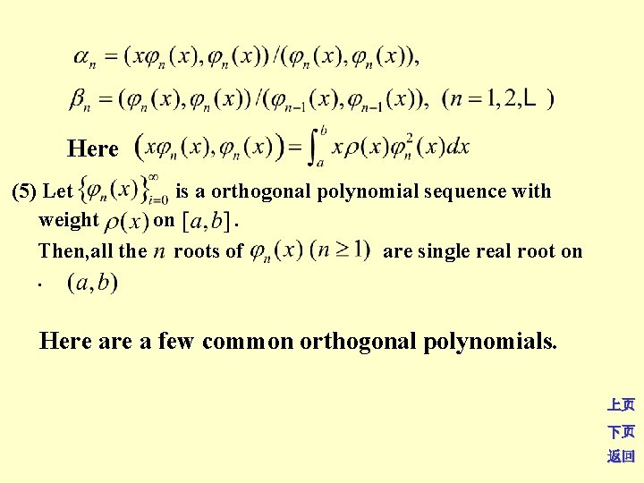
Here (5) Let is a orthogonal polynomial sequence with weight on . Then, all the roots of are single real root on . Here a few common orthogonal polynomials. 上页 下页 返回

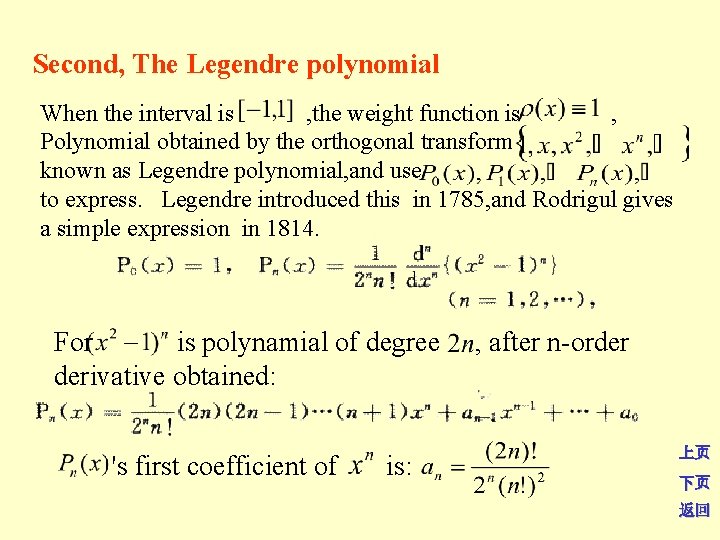
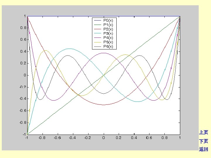
Second, The Legendre polynomial When the interval is , the weight function is , Polynomial obtained by the orthogonal transform known as Legendre polynomial, and use to express. Legendre introduced this in 1785, and Rodrigul gives a simple expression in 1814. For is polynamial of degree derivative obtained: 's first coefficient of is: , after n-order 上页 下页 返回

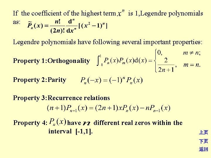
If the coefficient of the highest term as: is 1, Legendre polynomials have following several important properties: Property 1: Orthogonality Property 2: Parity Property 3: Recurrence relations Property 4: have different real zeros within the interval [-1, 1]. 上页 下页 返回

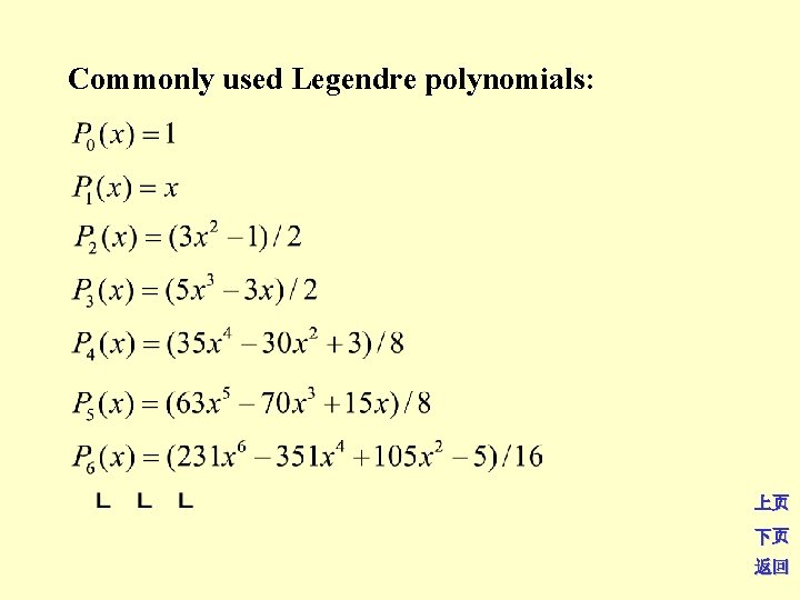
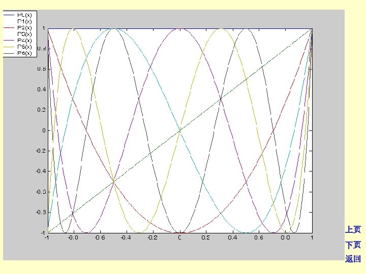
Commonly used Legendre polynomials: 上页 下页 返回

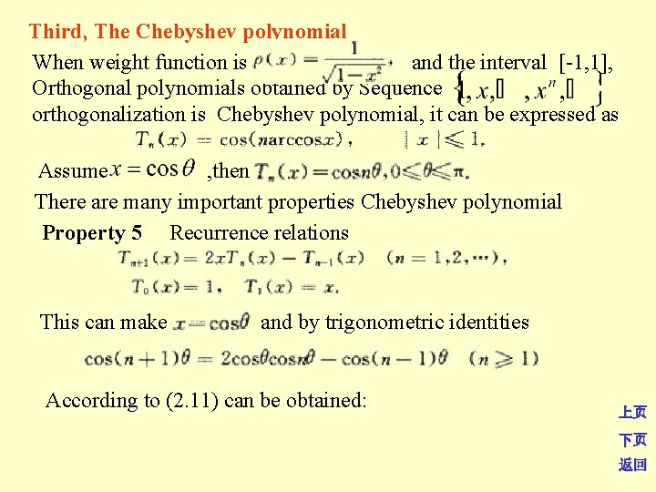
Third, The Chebyshev polynomial When weight function is and the interval [-1, 1], Orthogonal polynomials obtained by Sequence orthogonalization is Chebyshev polynomial, it can be expressed as Assume , then There are many important properties Chebyshev polynomial Property 5 Recurrence relations This can make and by trigonometric identities According to (2. 11) can be obtained: 上页 下页 返回

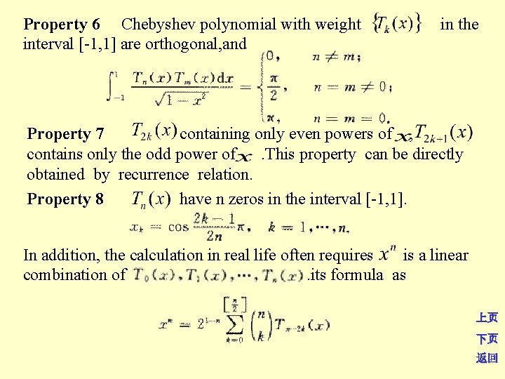
Property 6 Chebyshev polynomial with weight interval [-1, 1] are orthogonal, and in the Property 7 containing only even powers of , contains only the odd power of. This property can be directly obtained by recurrence relation. Property 8 have n zeros in the interval [-1, 1]. In addition, the calculation in real life often requires is a linear combination of. its formula as 上页 下页 返回

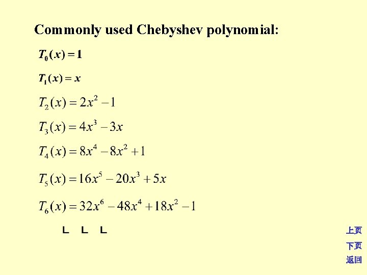
Commonly used Chebyshev polynomial: 上页 下页 返回

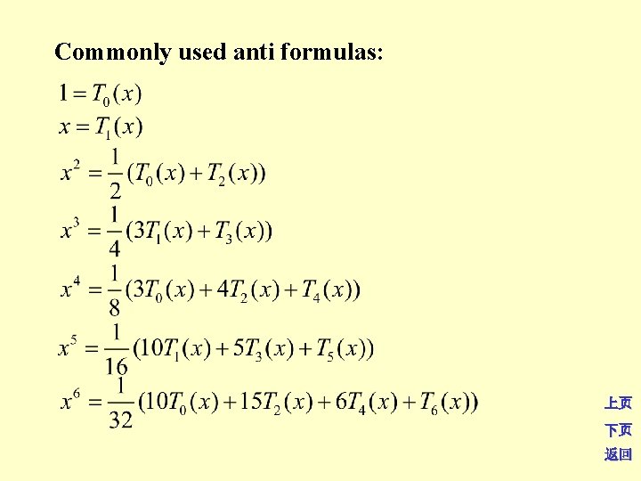
Commonly used anti formulas: 上页 下页 返回

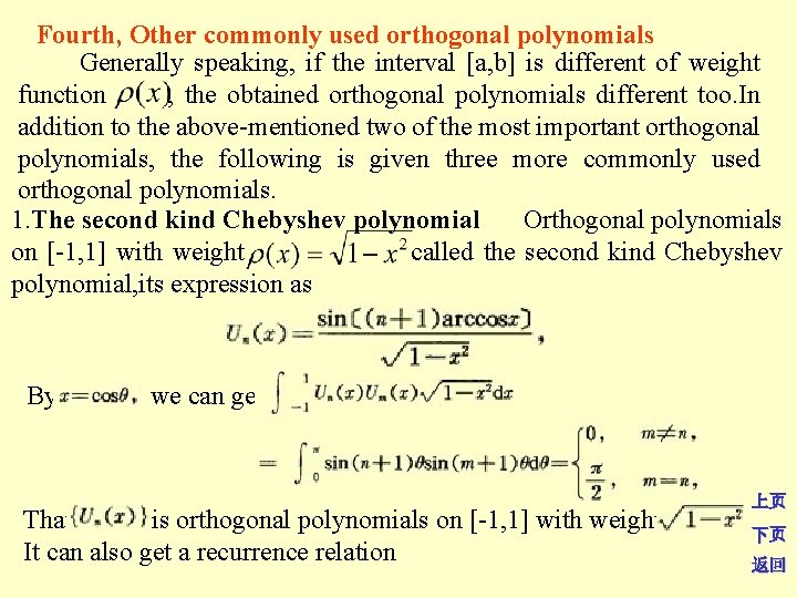
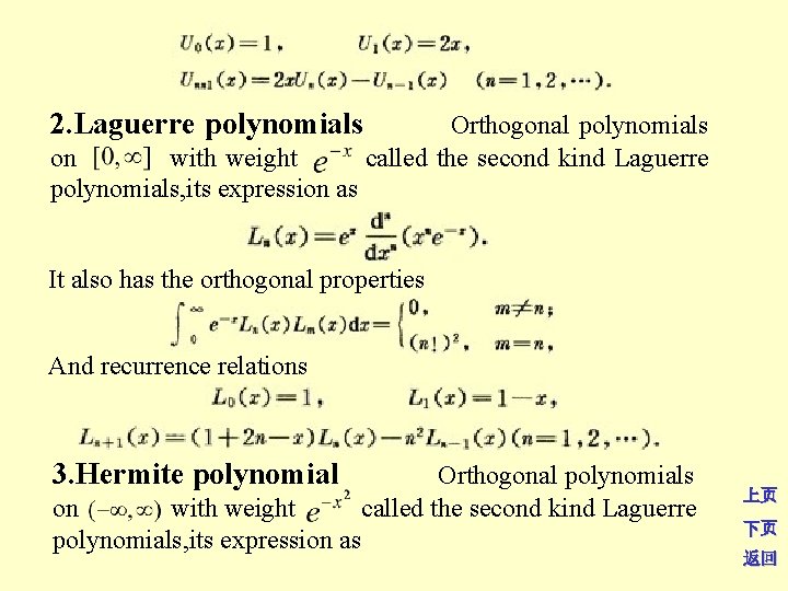
Fourth, Other commonly used orthogonal polynomials Generally speaking, if the interval [a, b] is different of weight function , the obtained orthogonal polynomials different too. In addition to the above-mentioned two of the most important orthogonal polynomials, the following is given three more commonly used orthogonal polynomials. 1. The second kind Chebyshev polynomial Orthogonal polynomials on [-1, 1] with weight called the second kind Chebyshev polynomial, its expression as By we can get That is orthogonal polynomials on [-1, 1] with weight It can also get a recurrence relation 上页 下页 返回

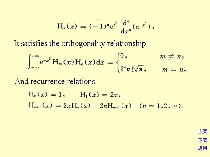
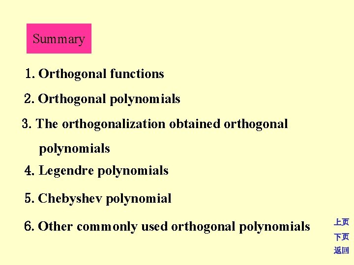
2. Laguerre polynomials Orthogonal polynomials on with weight called the second kind Laguerre polynomials, its expression as It also has the orthogonal properties And recurrence relations 3. Hermite polynomial Orthogonal polynomials on with weight called the second kind Laguerre polynomials, its expression as 上页 下页 返回

It satisfies the orthogonality relationship And recurrence relations 上页 下页 返回

Summary 1. Orthogonal functions 2. Orthogonal polynomials 3. The orthogonalization obtained orthogonal polynomials 4. Legendre polynomials 5. Chebyshev polynomial 6. Other commonly used orthogonal polynomials 上页 下页 返回

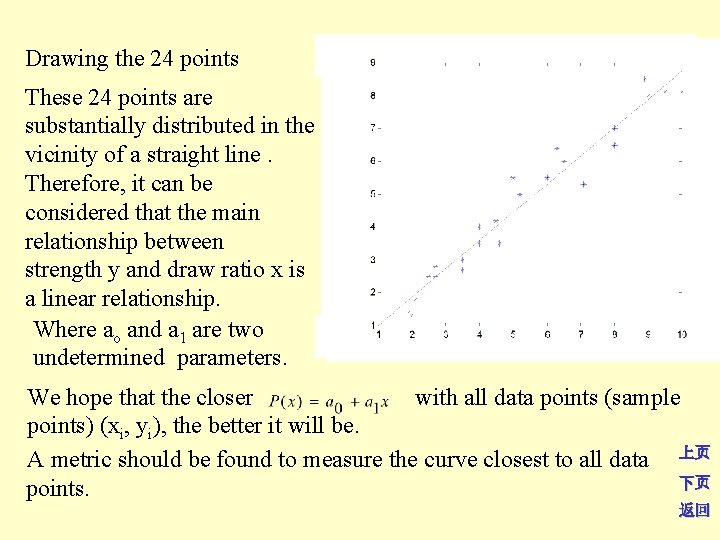
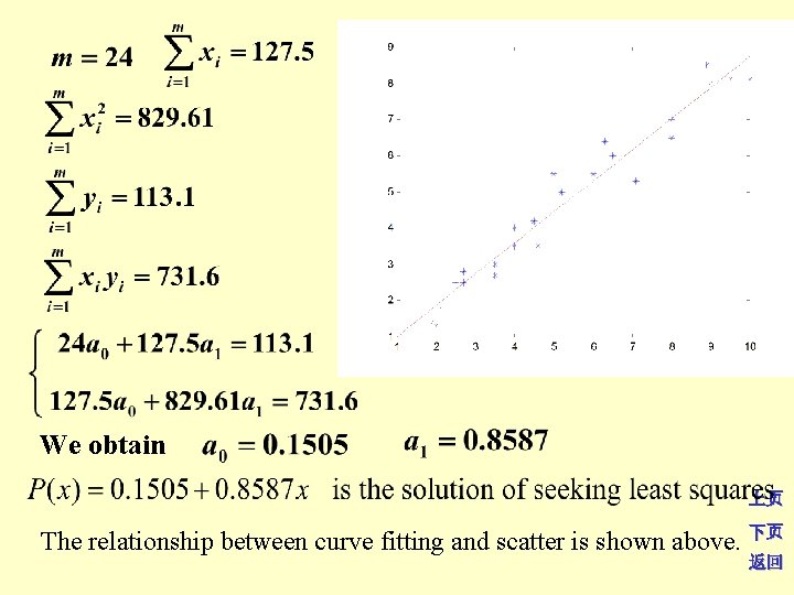
§ 8 Least squares method of curve fitting Instance: To investigate the relationship between strength of the fiber and its stretching ratio, the following table is the actually measured recording of the 24 fiber samples’strength and the corresponding draw ratio. 上页 The fiber strength is increased with the draw ratio. 下页 返回

Drawing the 24 points These 24 points are substantially distributed in the vicinity of a straight line. Therefore, it can be considered that the main relationship between strength y and draw ratio x is a linear relationship. Where ao and a 1 are two undetermined parameters. We hope that the closer with all data points (sample points) (xi, yi), the better it will be. A metric should be found to measure the curve closest to all data 上页 下页 points. 返回

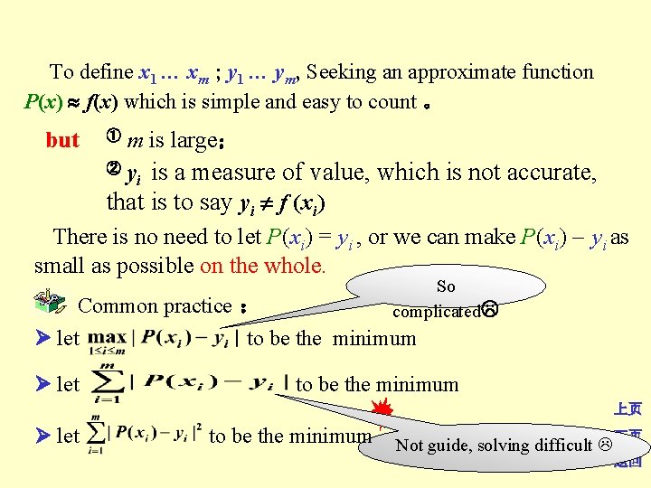
To define x 1 … xm ; y 1 … ym, Seeking an approximate function P(x) f(x) which is simple and easy to count 。 but m is large； ② y is a measure of value, which is not accurate, i that is to say yi f (xi) There is no need to let P(xi) = yi , or we can make P(xi) yi as small as possible on the whole. ① So complicated Common practice ： let to be the minimum let to be the minimum 上页 let to be the minimum Not guide, solving difficult 下页 返回

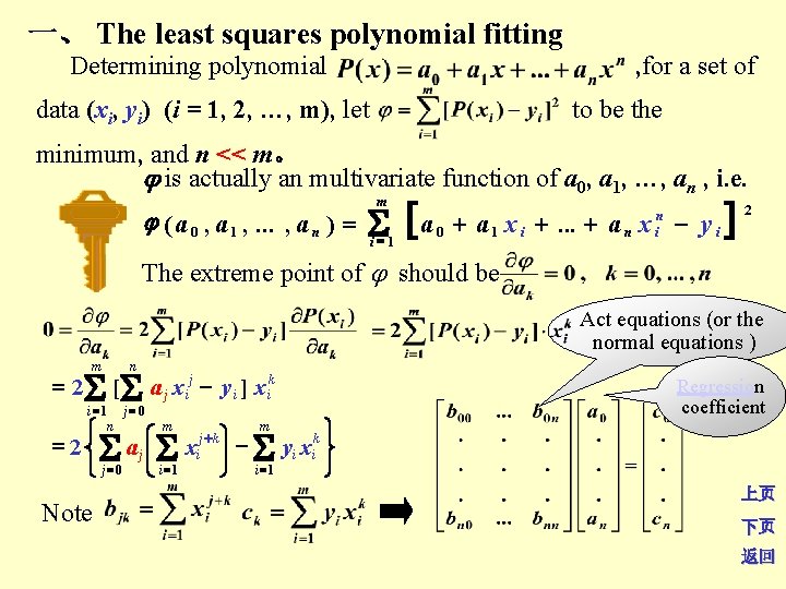
一、 The least squares polynomial fitting Determining polynomial , for a set of data (xi, yi) (i = 1, 2, …, m), let to be the minimum, and n << m。 is actually an multivariate function of a 0, a 1, …, an , i. e. ( a 0 , a 1 , . . . , a n ) = [a m i =1 0 + a 1 x i +. . . + a n x in y i ] 2 The extreme point of should be Act equations (or the normal equations ) =2 m n [ i =1 =2 j=0 n m j =0 Note a j x ij y i ] x ik aj i =1 x j+k i m i =1 Regression coefficient yi xik 上页 下页 返回

there exist the only least squares polynomial fitting (n < m). Theorem Solutions of Ba = c is indeed the minimum point of the Theorem n bj x . let a is a solution，then corresponding polynomial F( x) = j =0 j of any b = (b 0 b 1 m… bn )T , there must be, m (a ) = [ P ( xi ) yi ]2 [ F ( xi ) yi ]2 = (b) i =1 m m (b) (a ) = [ F ( x i ) yi ] [ P ( xi ) yi ]2 Proof： 2 i =1 m m = [F ( xi ) P( xi ) + P( xi ) yi ] [ P( xi ) yi ]2 i =1 m = [F ( xi ) P( xi )] + 2 [F ( xi ) P( xi )][P( xi ) yi ] i =1 2 i =1 0 Note： Least squares method requires to set the form of P (x). 上页 下页 P (x) is not necessarily a polynomial, but usually 返回 determined empirically. 上页

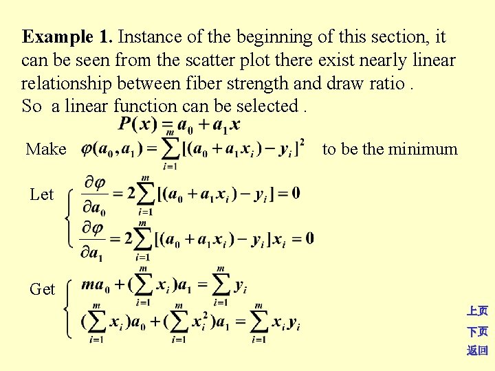
Example 1. Instance of the beginning of this section, it can be seen from the scatter plot there exist nearly linear relationship between fiber strength and draw ratio. So a linear function can be selected. Make to be the minimum Let Get 上页 下页 返回

We obtain 上页 The relationship between curve fitting and scatter is shown above. 下页 返回

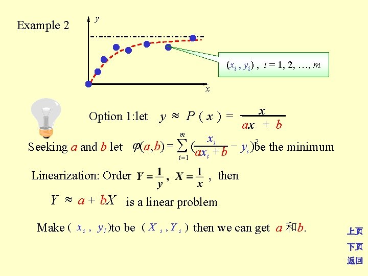
Example 2 y (xi , yi) , i = 1, 2, …, m x Option 1: let y P ( x ) = m x x ax + b 2 Seeking a and b let (a, b) = (ax +i b yi )be the minimum i i =1 Linearization: Order , then Y a + b. X is a linear problem Make ( x i , y I )to be ( X i , Y i ) then we can get a 和b. 上页 下页 返回

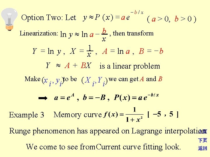
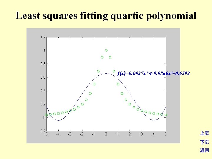
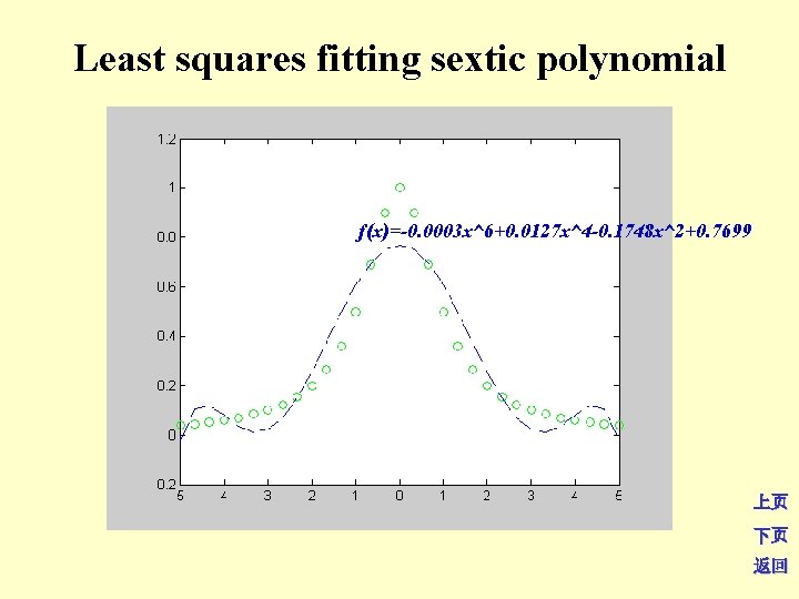
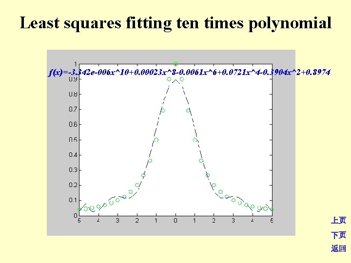
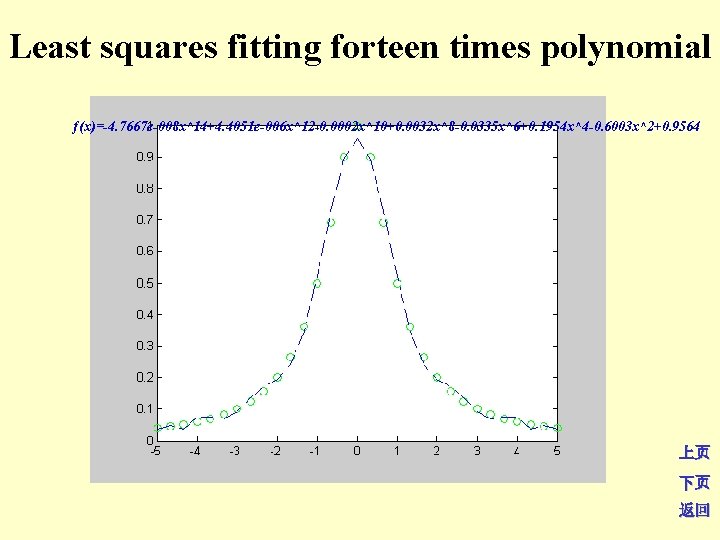
Option Two: Let y P ( x ) = a e b/ x ( a > 0, b > 0 ) Linearization: ln y ln a b , then transform x Y = ln y , X = x 1 , A = ln a , B = b Y A + BX is a linear problem Make (x , y )to be ( X , Y ) we can get A and B i i Example 3 i i Memory curve 上页 Runge phenomenon has appeared on Lagrange interpolation We come to see from. Current curve fitting look. 下页 返回

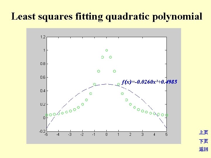
Least squares fitting quadratic polynomial ƒ(x)=-0. 0260 x²+0. 4985 上页 下页 返回

Least squares fitting quartic polynomial ƒ(x)=0. 0027 x^4 -0. 0866 x²+0. 6593 上页 下页 返回

Least squares fitting sextic polynomial ƒ(x)=-0. 0003 x^6+0. 0127 x^4 -0. 1748 x^2+0. 7699 上页 下页 返回

Least squares fitting ten times polynomial ƒ(x)=-3. 342 e-006 x^10+0. 00023 x^8 -0. 0061 x^6+0. 0721 x^4 -0. 3904 x^2+0. 8974 上页 下页 返回

Least squares fitting forteen times polynomial ƒ(x)=-4. 7667 e-008 x^14+4. 4051 e-006 x^12 -0. 0002 x^10+0. 0032 x^8 -0. 0335 x^6+0. 1954 x^4 -0. 6003 x^2+0. 9564 上页 下页 返回

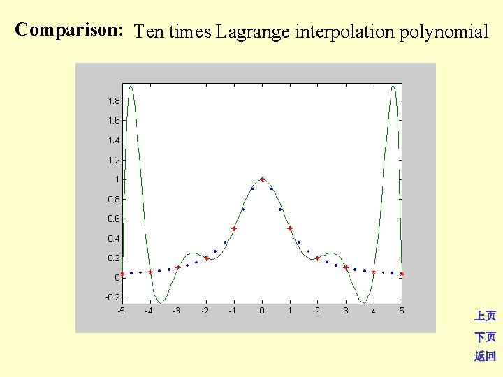
Comparison: Ten times Lagrange interpolation polynomial 上页 下页 返回

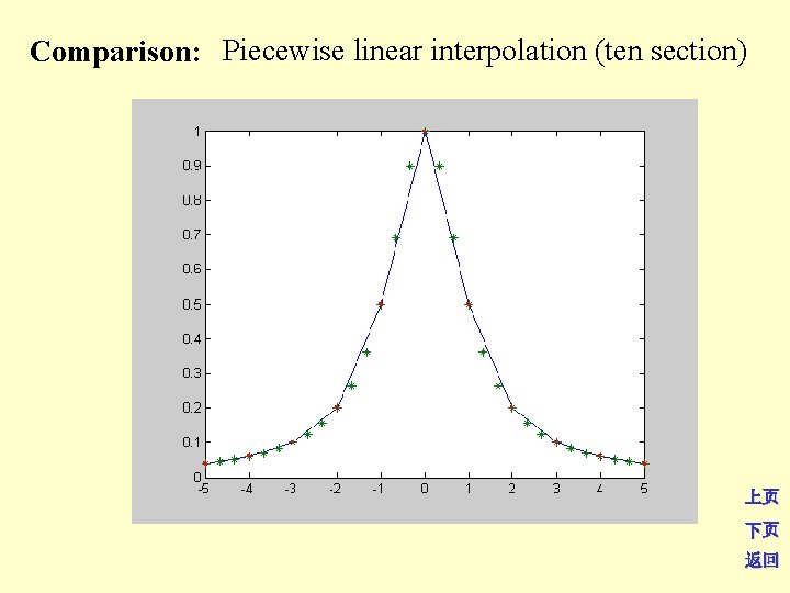
Comparison: Piecewise linear interpolation (ten section) 上页 下页 返回

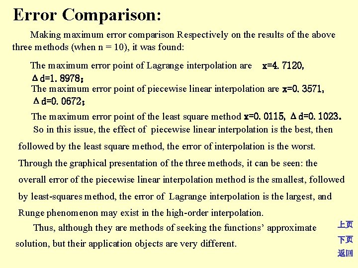
Error Comparison: Making maximum error comparison Respectively on the results of the above three methods (when n = 10), it was found: The maximum error point of Lagrange interpolation are x=4. 7120, Δd=1. 8978； The maximum error point of piecewise linear interpolation are x=0. 3571, Δd=0. 0672； The maximum error point of the least square method x=0. 0115, Δd=0. 1023. So in this issue, the effect of piecewise linear interpolation is the best, then followed by the least square method, the error of interpolation is the worst. Through the graphical presentation of the three methods, it can be seen: the overall error of the piecewise linear interpolation method is the smallest, followed by least-squares method, the error of Lagrange interpolation is the largest, and Runge phenomenon may exist in the high-order interpolation. Thus, although they are methods of seeking the functions’ approximate solution, but their application objects are very different. 上页 下页 返回

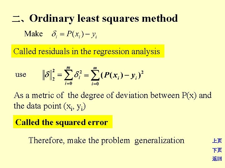
二、Ordinary least squares method Called residuals in the regression analysis use As a metric of the degree of deviation between P(x) and the data point (xi, yi) Called the squared error Therefore, make the problem generalization 上页 下页 返回

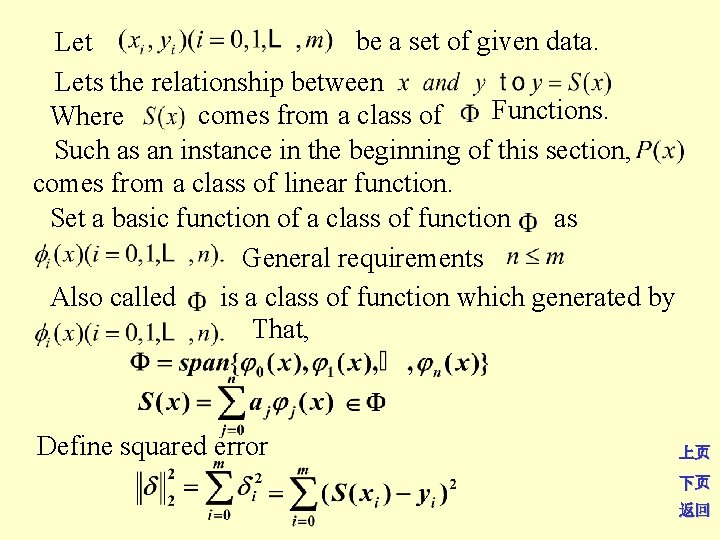
be a set of given data. Lets the relationship between Functions. comes from a class of Where Such as an instance in the beginning of this section, comes from a class of linear function. Set a basic function of a class of function as General requirements Also called is a class of function which generated by That, Define squared error 上页 下页 返回

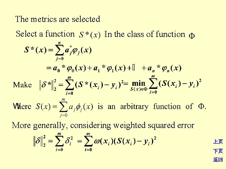
The metrics are selected Select a function In the class of function More generally, considering weighted squared error 上页 下页 返回

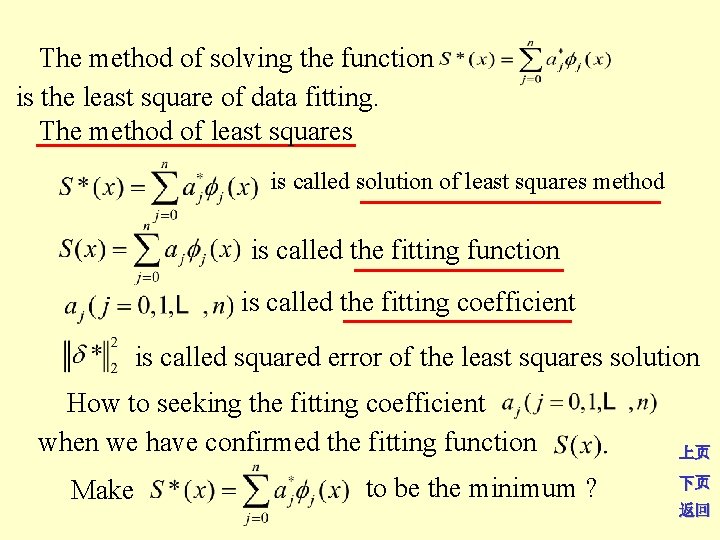
The method of solving the function is the least square of data fitting. The method of least squares is called solution of least squares method is called the fitting function is called the fitting coefficient is called squared error of the least squares solution How to seeking the fitting coefficient when we have confirmed the fitting function Make to be the minimum ? 上页 下页 返回

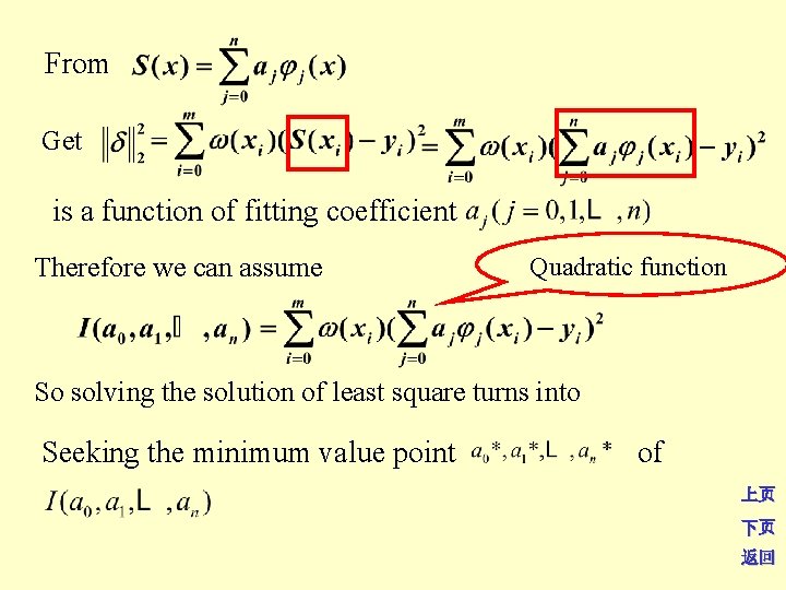
From Get is a function of fitting coefficient Therefore we can assume Quadratic function So solving the solution of least square turns into Seeking the minimum value point of 上页 下页 返回

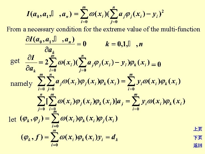
From a necessary condition for the extreme value of the multi-function get namely let 上页 下页 返回

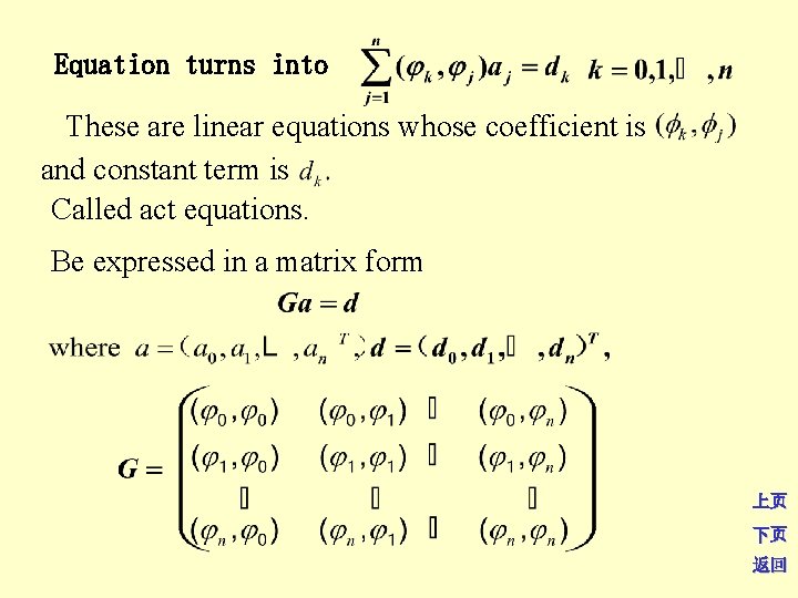
Equation turns into These are linear equations whose coefficient is and constant term is Called act equations. Be expressed in a matrix form 上页 下页 返回

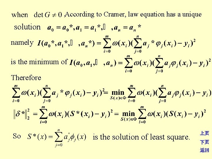
According to Cramer, law equation has a unique solution namely is the minimum of Therefore So is the solution of least square. 上页 下页 返回

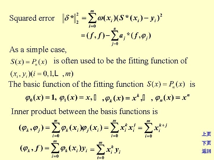
Squared error As a simple case, is often used to be the fitting function of The basic function of the fitting function is Inner product between the basis functions is 上页 下页 返回

Summary 1. Least squares method of curve fitting 2. The least squares polynomial fitting 3. Ordinary least squares method 上页 下页 返回

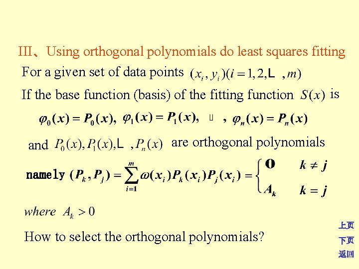
III、Using orthogonal polynomials do least squares fitting For a given set of data points If the base function (basis) of the fitting function and is are orthogonal polynomials namely How to select the orthogonal polynomials? 上页 下页 返回

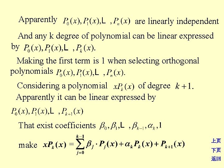
Apparently are linearly independent And any k degree of polynomial can be linear expressed by Making the first term is 1 when selecting orthogonal polynomials Considering a polynomial of degree Apparently it can be linear expressed by That exist coefficients make 上页 下页 返回

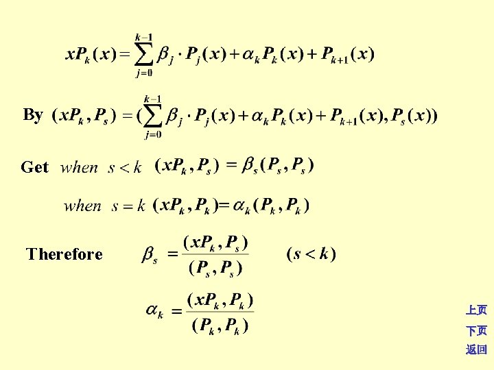
By Get Therefore 上页 下页 返回

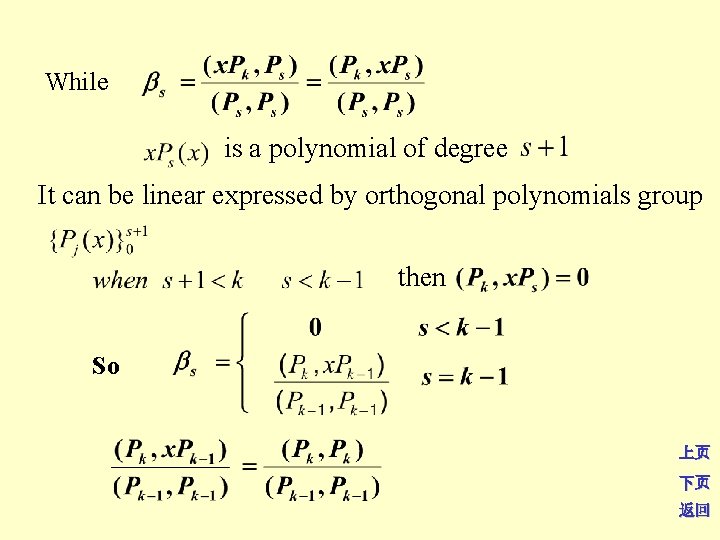
While is a polynomial of degree It can be linear expressed by orthogonal polynomials group then So 上页 下页 返回

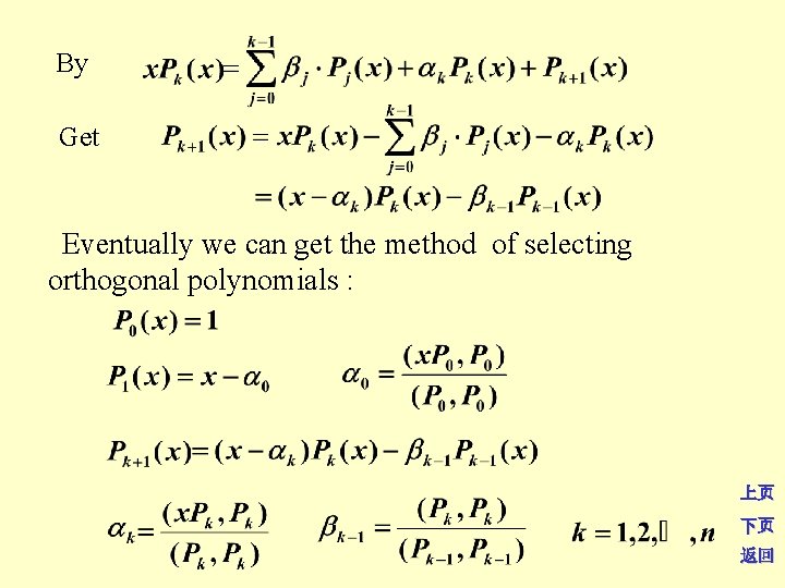
By Get Eventually we can get the method of selecting orthogonal polynomials : 上页 下页 返回

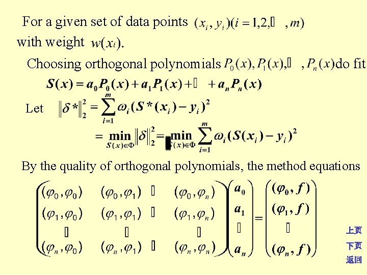
For a given set of data points with weight Choosing orthogonal polynomials do fit Let By the quality of orthogonal polynomials, the method equations 上页 下页 返回

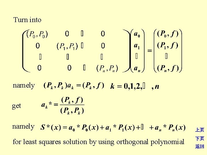
Turn into namely get namely for least squares solution by using orthogonal polynomial 上页 下页 返回

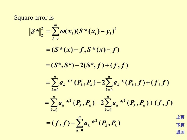
Square error is 上页 下页 返回

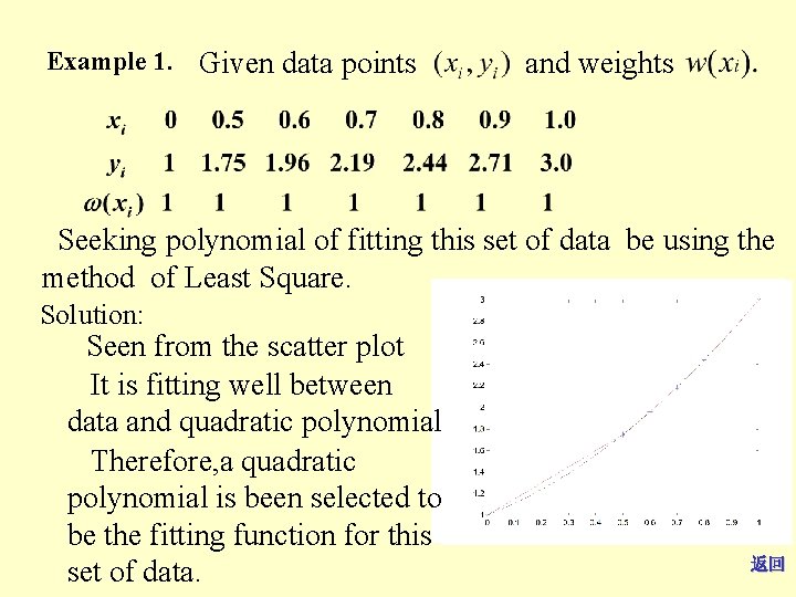
Example 1. Given data points and weights Seeking polynomial of fitting this set of data be using the method of Least Square. Solution: Seen from the scatter plot It is fitting well between data and quadratic polynomial Therefore, a quadratic polynomial is been selected to be the fitting function for this set of data. 上页 下页 返回

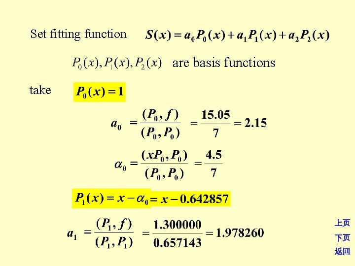
Set fitting function are basis functions take 上页 下页 返回

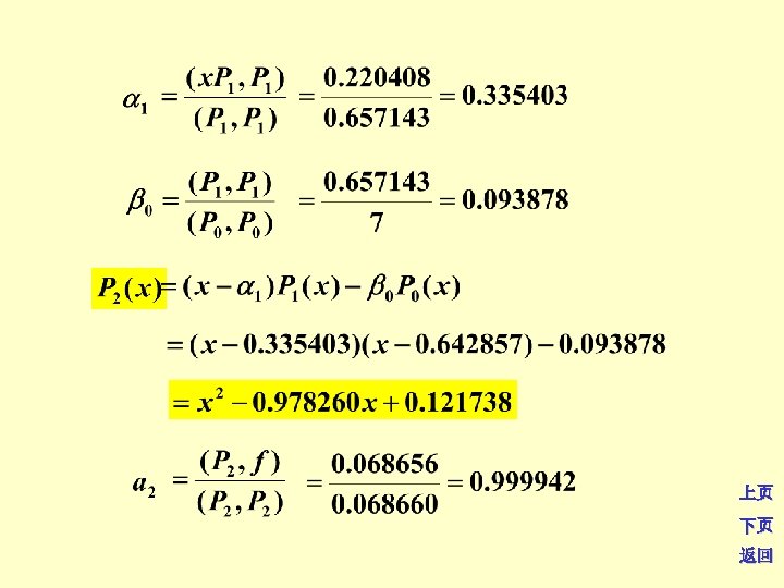
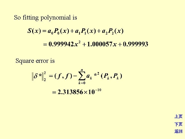
So fitting polynomial is Square error is 上页 下页 返回

Summary 1 、Fitting least squares by using orthogonal polynomial. 上页 下页 返回

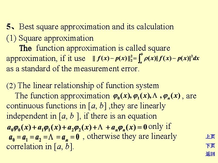
5、Best square approximation and its calculation (1) Square approximation The function approximation is called square approximation, if it use as a standard of the measurement error. (2) The linear relationship of function system The function approximation , are continuous functions in [a, b] , they are linearly independent in [a, b ], if there is an equation only if , otherwise they are linearly correlation in [a, b]. 上页 下页 返回

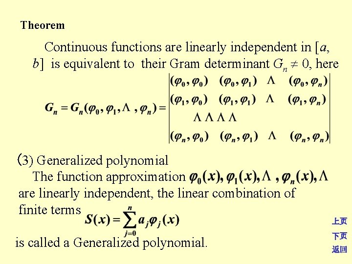
Theorem Continuous functions are linearly independent in [a, b] is equivalent to their Gram determinant Gn 0, here (3) Generalized polynomial The function approximation are linearly independent, the linear combination of finite terms 上页 is called a Generalized polynomial. 下页 返回

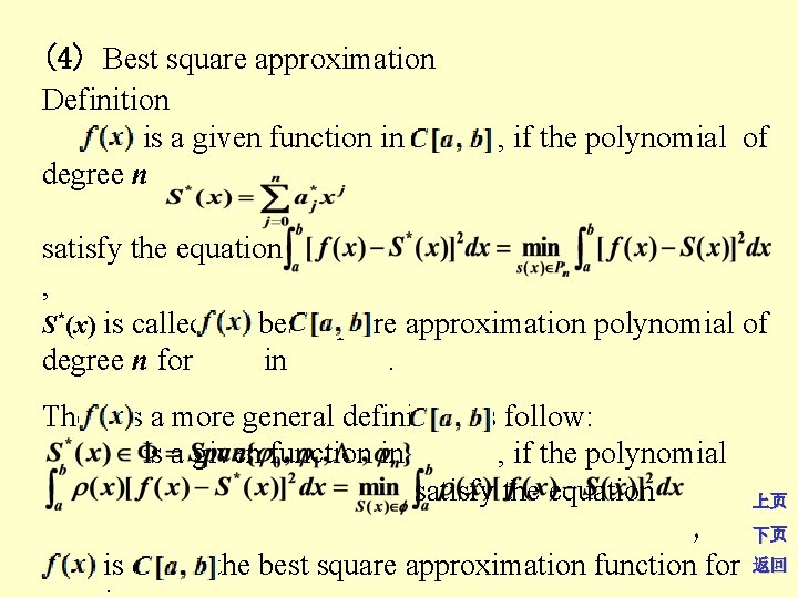
(4) Best square approximation Definition is a given function in degree n , if the polynomial of satisfy the equation , S*(x) is called the best square approximation polynomial of degree n for in. There is a more general definition as follow: is a given function in , if the polynomial satisfy the equation , S*(x) is called the best square approximation function for 上页 下页 返回

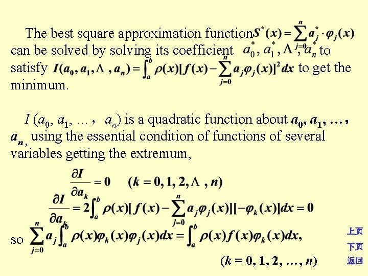
The best square approximation function can be solved by solving its coefficient satisfy minimum. to to get the I (a 0, a 1, …，an) is a quadratic function about a 0, a 1, …， an , using the essential condition of functions of several variables getting the extremum, 上页 so 下页 (k = 0, 1, 2, …, n) 返回

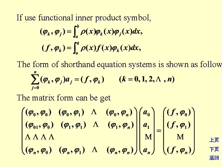
If use functional inner product symbol, The form of shorthand equation systems is shown as follow The matrix form can be get 上页 下页 返回

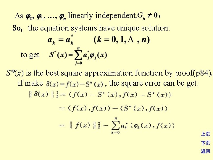
As 0, 1, …, n linearly independent, Gn 0， So, the equation systems have unique solution: to get S*(x) is the best square approximation function by proof(p 84). if make , the square error can be get: 上页 下页 返回

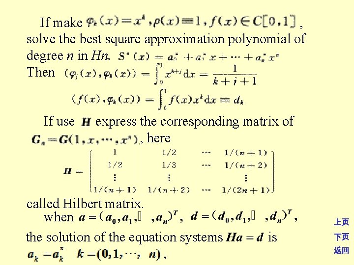
If make , solve the best square approximation polynomial of degree n in Hn, Then If use express the corresponding matrix of , here called Hilbert matrix. when the solution of the equation systems. 上页 is 下页 返回

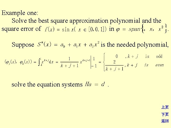
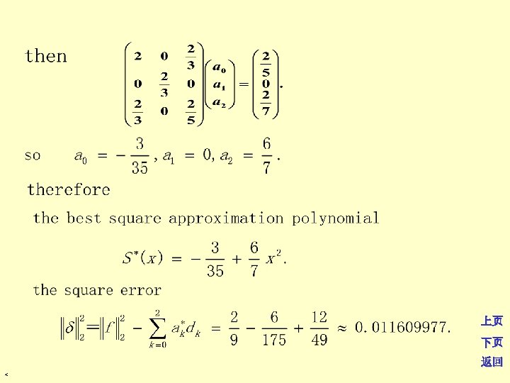
Example one: Solve the best square approximation polynomial and the square error of in. Suppose solve the equation systems is the needed polynomial, . 上页 下页 返回

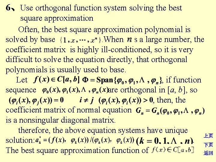
6、Use orthogonal function system solving the best square approximation Often, the best square approximation polynomial is solved by base. When is a large number, the coefficient matrix is highly ill-conditioned, so it is very difficult to solve the equation directly, that orthogonal polynomials is usually used to base. Let , , if function sequence are orthogonal in [a, b], so , then, the coefficient matrix of normal equation is a nonsingular diagonal matrix. therefore, the above equation systems have unique 上页 solution: . 下页 The best square approximation function of 返回

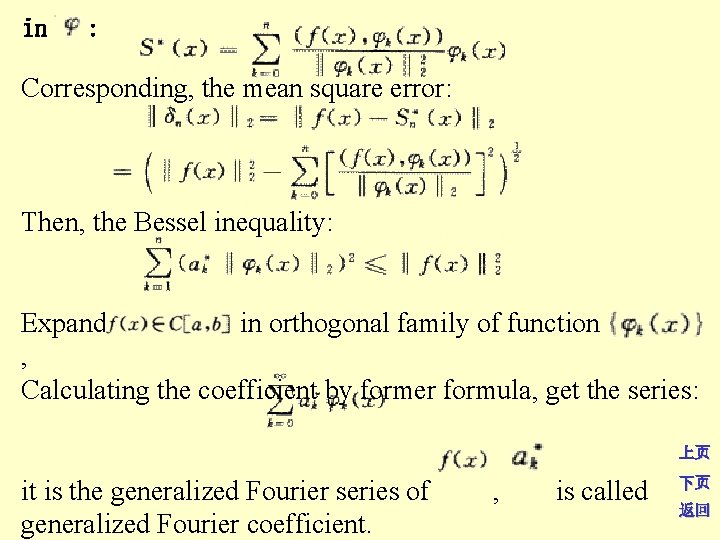
in : Corresponding, the mean square error: Then, the Bessel inequality: Expand in orthogonal family of function , Calculating the coefficient by former formula, get the series: 上页 it is the generalized Fourier series of generalized Fourier coefficient. , is called 下页 返回

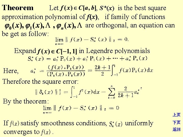
Theorem Let , S*(x) is the best square approximation polynomial of f(x), if family of functions are orthogonal, an equation can be get as follow: Expand in Legendre polynomials Here, Therefore the square error: By theorem: 上页 If satisfy smoothness conditions, converges to. uniformly 下页 返回

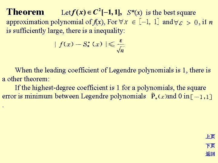
Theorem Let S*(x) is the best square approximation polynomial of f(x), For and , if is sufficiently large, there is a inequality: When the leading coefficient of Legendre polynomials is 1, there is a other theorem: If the highest-degree coefficient is 1 for a polynomials, the square error is minimum between Legendre polynomials and 0 in. 上页 下页 返回

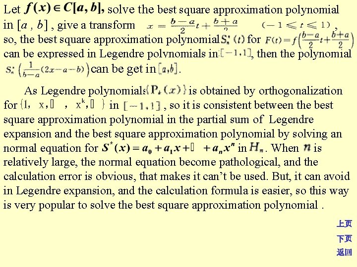
Let solve the best square approximation polynomial in [a , b] , give a transform , so, the best square approximation polynomial can be expressed in Legendre polynomials in can be get in for , then the polynomial . As Legendre polynomials is obtained by orthogonalization for in , so it is consistent between the best square approximation polynomial in the partial sum of Legendre expansion and the best square approximation polynomial by solving an normal equation for in. When is relatively large, the normal equation become pathological, and the calculation error is obvious, that makes it can’t be used. But, it can avoid in Legendre expansion, and the calculation formula is easier, so this way is very popular to solve the best square approximation polynomial. 上页 下页 返回

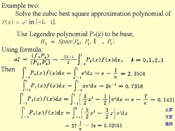
Example two: Solve the cubic best square approximation polynomial of in. Use Legendre polynomial Pn(x) to be base, Using formula: Then 上页 下页 返回

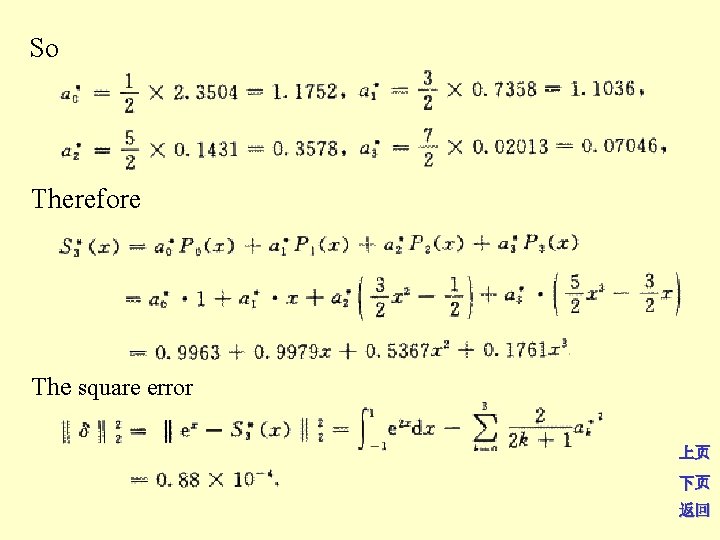
So Therefore The square error 上页 下页 返回

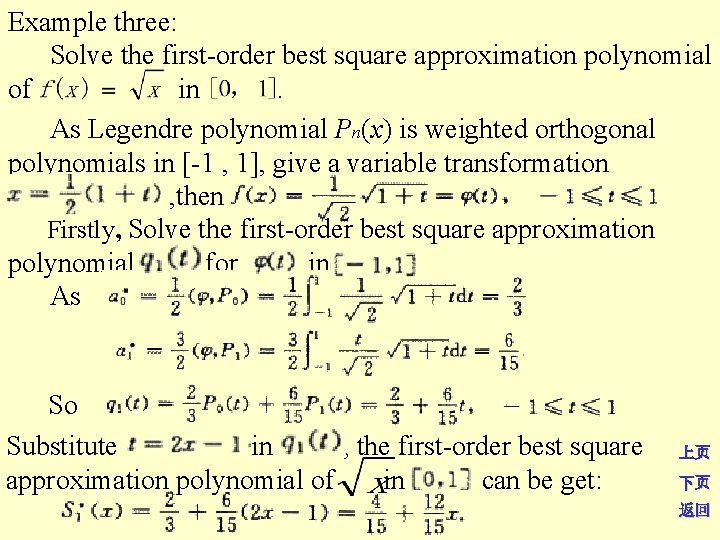
Example three: Solve the first-order best square approximation polynomial of in. As Legendre polynomial Pn(x) is weighted orthogonal polynomials in [-1 , 1], give a variable transformation , then Firstly, Solve the first-order best square approximation polynomial for in , As So Substitute in , the first-order best square approximation polynomial of in can be get: 上页 下页 返回

Summary 1. Square approximation 2．Linear relationship of function system 3．Generalized polynomials 4. Best square approximation 5. Get the best square approximation by orthogonal family of function 上页 下页 返回