Numerical Analysis Lecture 42 Examples of Numerical Differentiation

Numerical Analysis Lecture 42

Examples of Numerical Differentiation

The simplest formula for differentiation is

Example Let f(x)= In x and x 0 = 1. 8. Then the quotient is used to approximate

with error where Let us see the results for h = 0. 1, 0. 01, and 0. 001.

h f(1. 8 + h) 0. 1 0. 64185389 0. 5406722 0. 0154321 0. 01 0. 59332685 0. 5540180 0. 0015432 0. 001 0. 58834207 0. 5554013 0. 0001543

Since The exact value of is and the error bounds are a appropriate.

The following two three point formulas become especially useful if the nodes are equally spaced, that is, when x 1 = x 0 + h and x 2 = x 0 + 2 h ,

where and lies between x 0 and x 0 + 2 h,

where lies between (x 0 – h) and (x 0 + h).

Given in Table below are values for f (x) = xex. x 1. 8 1. 9 2. 0 2. 1 2. 2 f (x) 10. 889365 12. 703199 14. 778112 17. 148957 19. 855030

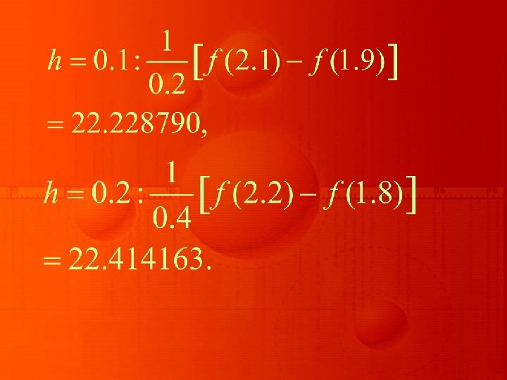
Since Approximating using the various three-and five-point formulas produces the following results.

Three point formulas:

Using three point formulas we get

Five point formula Using the five point formula with h = 0. 1 (the only formula applicable):

The errors in the formulas are approximately and respectively. Clearly, the five-point formula gives the superior result.

Consider approximating for f (x) = sin x, using the values in table [ the true value is cos (0. 900) = 0. 62161. ] x 0. 800 0. 850 0. 880 0. 895 0. 898 0. 899 sin x 0. 71736 0. 75128 0. 77074 0. 77707 0. 78021 0. 78208 0. 78270 x 0. 901 0. 902 0. 905 0. 910 0. 920 0. 950 1. 000 sin x 0. 78395 0. 78457 0. 78643 0. 78950 0. 79560 0. 81342 0. 84147

Using the formula with different values of h gives the approximations in table given below:

h Approximation Error to 0. 001 0. 002 0. 005 0. 010 0. 020 0. 050 0. 100 0. 62500 0. 62250 0. 62200 0. 62150 0. 62140 0. 62055 0. 00339 0. 00089 0. 00039 -0. 00011 -0. 00021 -0. 00106

Examples of Numerical Integration

EXAMPLE The Trapezoidal rule for a function f on the interval [0, 2] is while Simpson’s rule for f on [0, 2] is

That is

f ( x) x 2 x 4 1/(x + 1) sin x ex Exact value 2. 667 6. 400 1. 099 2. 958 1. 416 6. 389 Trapezoidal 4. 000 16. 000 1. 333 3. 326 0. 909 8. 389 Simpson’s 2. 667 6. 667 1. 111 2. 964 1. 425 6. 421

Use close and open formulas listed below to approximate

Some of the common closed Newton-Cotes formulas with their error terms are as follows: n = 1: where Trapezoidal rule

n = 2: Simpson’s rule n = 3: Simpson’s rule

n = 4: where n = 0: Midpoint rule where

n 1 2 3 4 Closed formulas 0. 27768018 0. 2929326 0. 29291 0. 2928 4 070 9318 Error 0. 01521303 0. 0000394 0. 00001 0. 0000 2 748 0004 Open formulas 0. 29798754 0. 2928586 0. 29286 6 923 Error 0. 00509432 0. 0000345 0. 00002 6 399

Composite Numerical Integration EXAMPLE 1 Consider approximating with an absolute error less than 0. 00002, using the Composite Simpson’s rule. The Composite Simpson’s rule gives

Since the absolute error is required to be less than 0. 00002, the inequality

is used to determine n and h. Computing these calculations gives n greater than or equal to 18. If n = 20, then the formula becomes

To be assured of this degree of accuracy using the Composite Trapezoidal rule requires that or that Since this is many more calculations than are needed for the Composite Simpson’s rule, it is clear that it

would be undesirable to use the Composite Trapezoidal rule on this problem. For comparison purposes, the Composite Trapezoidal rule with n = 20 and gives

The exact answer is 2; so Simpson’s rule with n = 20 gave an answer well within the required error bound, whereas the Trapezoidal rule with n = 20 clearly did not.

An Example of Industrial applications: A company advertises that every roll of toilet paper has at least 250 sheets. The probability that there are 250 or more sheets in the toilet paper is given by

Approximating the above integral as a)use single segment Trapezoidal rule to find the probability that there are 250 or more sheets. b)Find the true error, Et for part (a). C)Find the absolute relative true error for part (a).

, where

b) The exact value of the above integral cannot be found. We assume the value obtained by adaptive numerical integration using Maple as the exact value for calculating the true error and relative true error. so the true error is

The absolute relative true error, , would then be

Improper Integrals EXAMPLE To approximate the values of the improper integral we will use the Composite Simpson’s rule with h = 0. 25. Since the fourth Taylor polynomial for ex about x = 0 is

We have

Table below lists the approximate values of x 0. 00 0. 25 0. 50 0. 75 1. 00 G(x) 0 0. 0000170 0. 0004013 0. 0026026 0. 0099485

Applying the Composite Simpson’s rule to G using these data gives Hence

This result is accurate within the accuracy of the Composite Simpson’s rule approximation for the function G. Since on [0, 1], the error is bounded by

EXAMPLE To approximate the value of the improper integral we make the change of variable t = x-1 to obtain The fourth Taylor polynomial, P 4(t), for sin t about 0 is

So we have Applying the Composite Simpson’s rule with n = 8 to the remaining integral gives which is accurate to within

Numerical Analysis Lecture 42