Numpy and Scipy Numerical Computing in Python 1

Numpy and Scipy Numerical Computing in Python 1

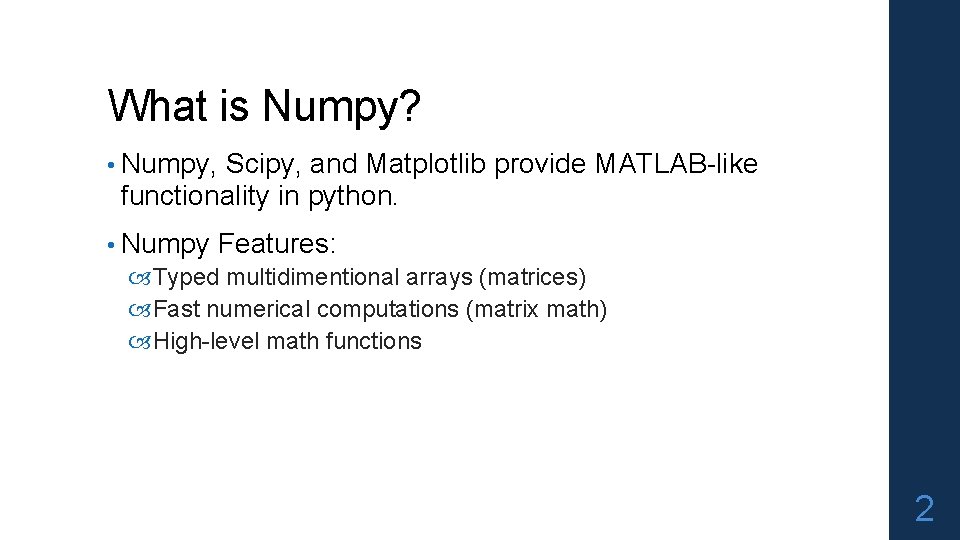
What is Numpy? • Numpy, Scipy, and Matplotlib provide MATLAB-like functionality in python. • Numpy Features: Typed multidimentional arrays (matrices) Fast numerical computations (matrix math) High-level math functions 2

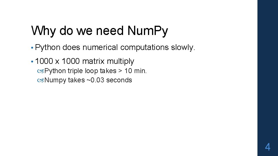
Why do we need Num. Py Let’s see for ourselves! 3

Why do we need Num. Py • Python does numerical computations slowly. • 1000 x 1000 matrix multiply Python triple loop takes > 10 min. Numpy takes ~0. 03 seconds 4

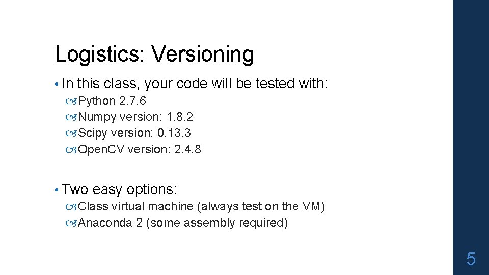
Logistics: Versioning • In this class, your code will be tested with: Python 2. 7. 6 Numpy version: 1. 8. 2 Scipy version: 0. 13. 3 Open. CV version: 2. 4. 8 • Two easy options: Class virtual machine (always test on the VM) Anaconda 2 (some assembly required) 5

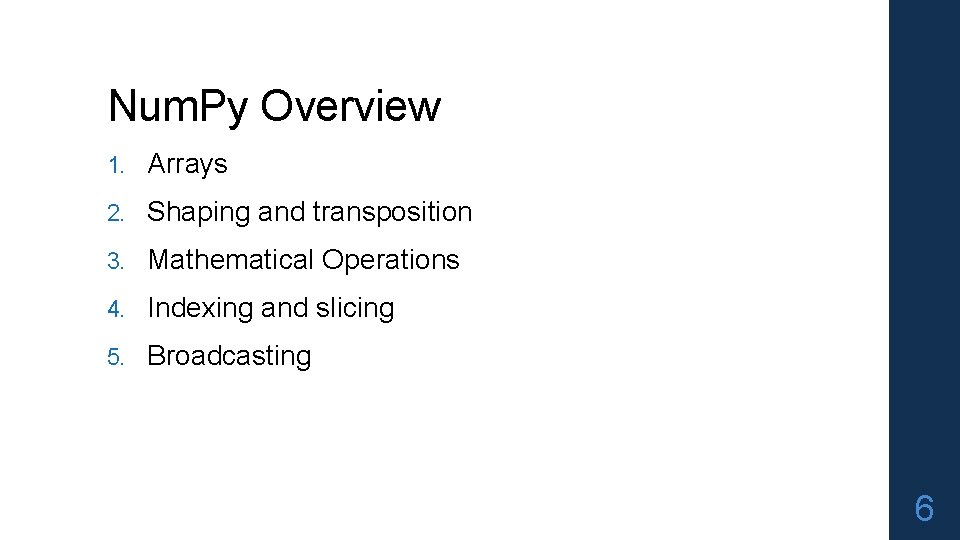
Num. Py Overview 1. Arrays 2. Shaping and transposition 3. Mathematical Operations 4. Indexing and slicing 5. Broadcasting 6

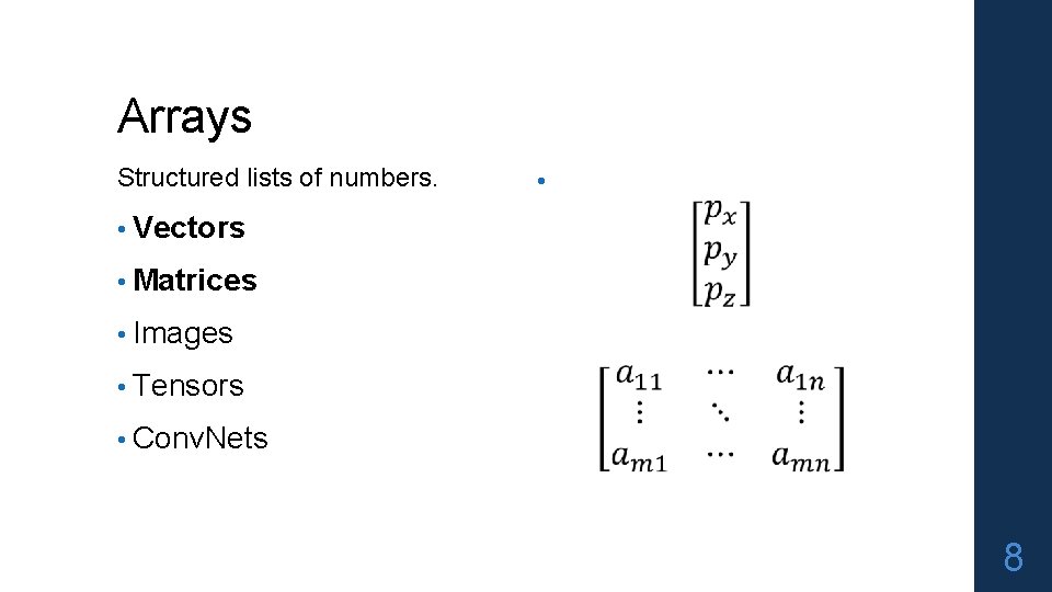
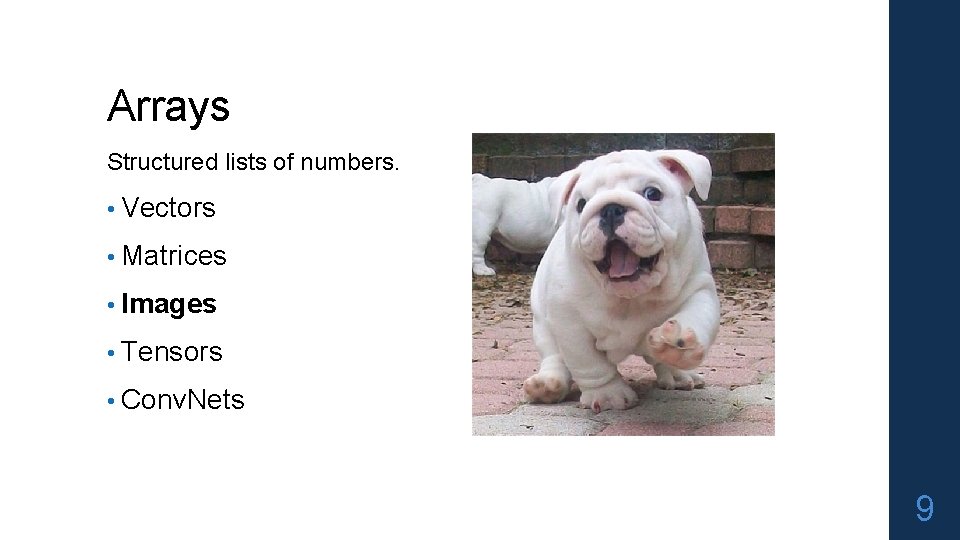
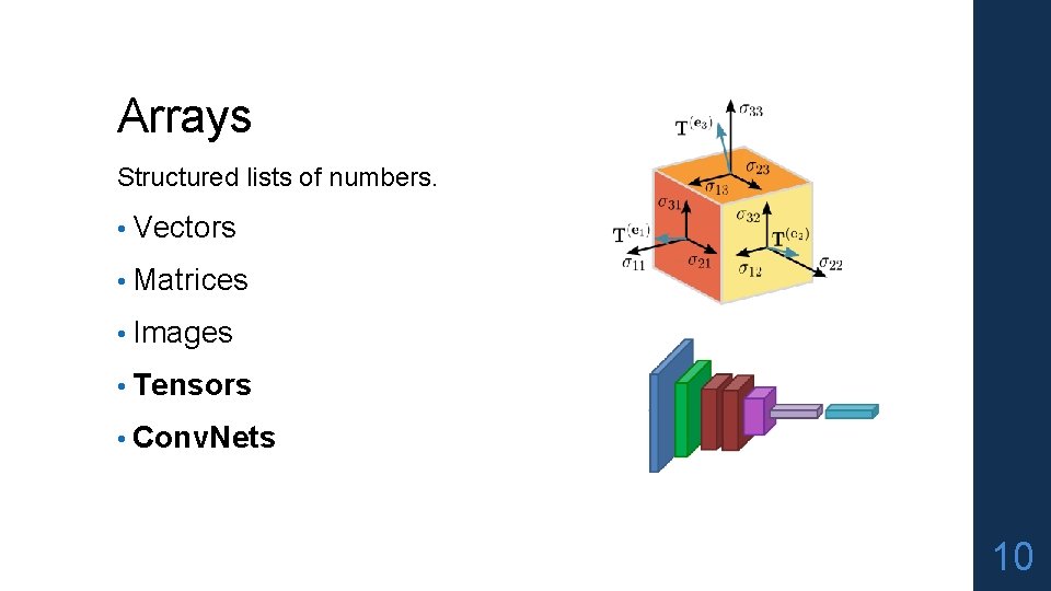
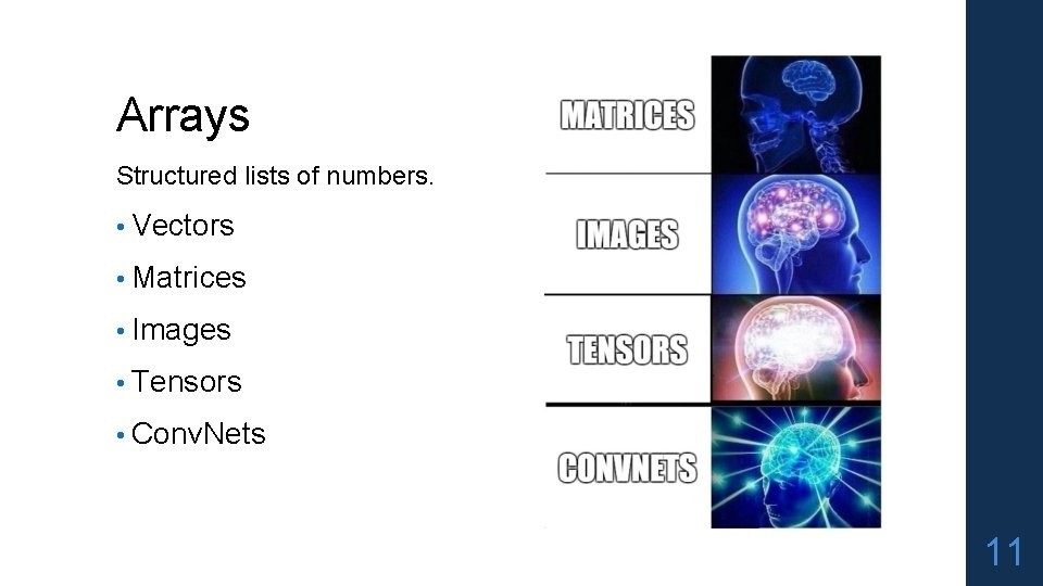
Arrays Structured lists of numbers. • Vectors • Matrices • Images • Tensors • Conv. Nets 7

Arrays Structured lists of numbers. • • Vectors • Matrices • Images • Tensors • Conv. Nets 8

Arrays Structured lists of numbers. • Vectors • Matrices • Images • Tensors • Conv. Nets 9

Arrays Structured lists of numbers. • Vectors • Matrices • Images • Tensors • Conv. Nets 10

Arrays Structured lists of numbers. • Vectors • Matrices • Images • Tensors • Conv. Nets 11

Arrays, Basic Properties import numpy as np a = np. array([[1, 2, 3], [4, 5, 6]], dtype=np. float 32) print a. ndim, a. shape, a. dtype 1. Arrays can have any number of dimensions, including zero (a scalar). 2. Arrays are typed: np. uint 8, np. int 64, np. float 32, np. float 64 3. Arrays are dense. Each element of the array exists and has the same type. 12

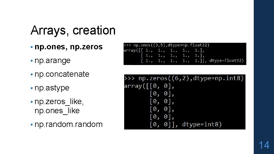
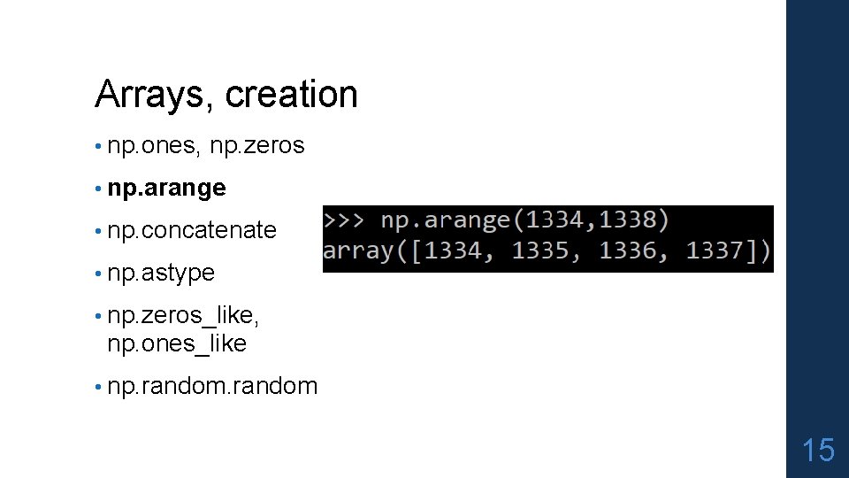
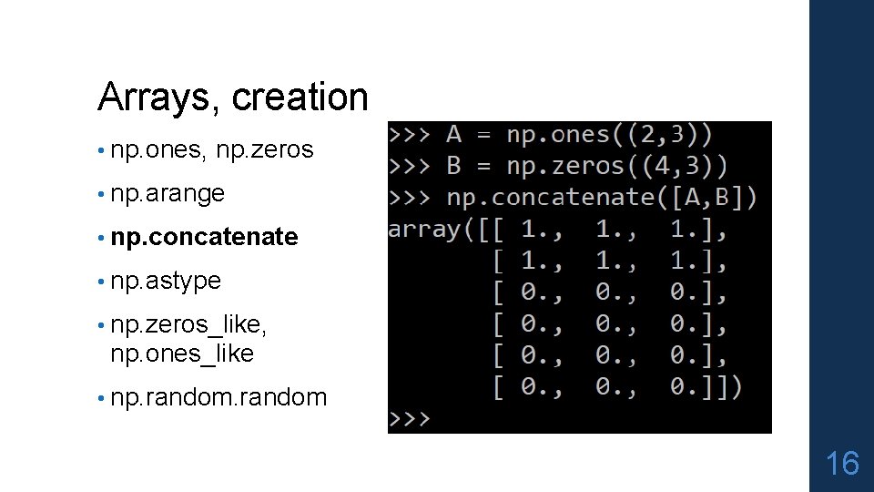
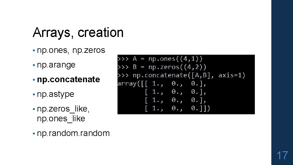
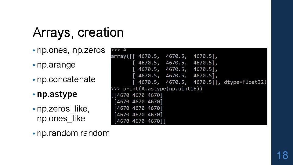
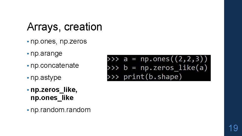
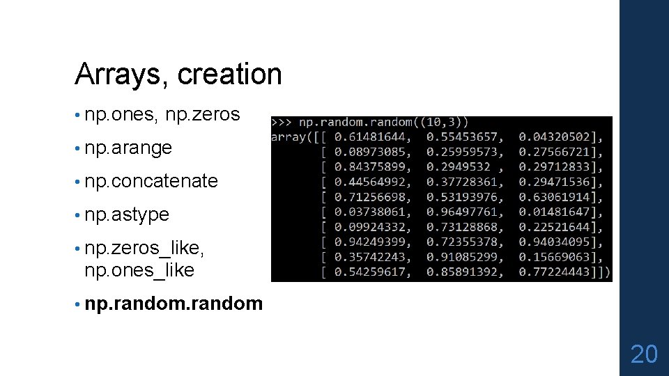
Arrays, creation • np. ones, np. zeros • np. arange • np. concatenate • np. astype • np. zeros_like, np. ones_like • np. random 13

Arrays, creation • np. ones, np. zeros • np. arange • np. concatenate • np. astype • np. zeros_like, np. ones_like • np. random 14

Arrays, creation • np. ones, np. zeros • np. arange • np. concatenate • np. astype • np. zeros_like, np. ones_like • np. random 15

Arrays, creation • np. ones, np. zeros • np. arange • np. concatenate • np. astype • np. zeros_like, np. ones_like • np. random 16

Arrays, creation • np. ones, np. zeros • np. arange • np. concatenate • np. astype • np. zeros_like, np. ones_like • np. random 17

Arrays, creation • np. ones, np. zeros • np. arange • np. concatenate • np. astype • np. zeros_like, np. ones_like • np. random 18

Arrays, creation • np. ones, np. zeros • np. arange • np. concatenate • np. astype • np. zeros_like, np. ones_like • np. random 19

Arrays, creation • np. ones, np. zeros • np. arange • np. concatenate • np. astype • np. zeros_like, np. ones_like • np. random 20

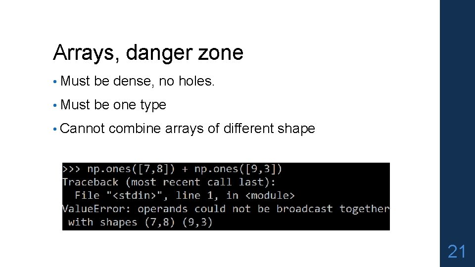
Arrays, danger zone • Must be dense, no holes. • Must be one type • Cannot combine arrays of different shape 21

Shaping a = np. array([1, 2, 3, 4, 5, 6]) a = a. reshape(3, 2) a = a. reshape(2, -1) a = a. ravel() 1. Total number of elements cannot change. 2. Use -1 to infer axis shape 3. Row-major by default (MATLAB is column-major) 22

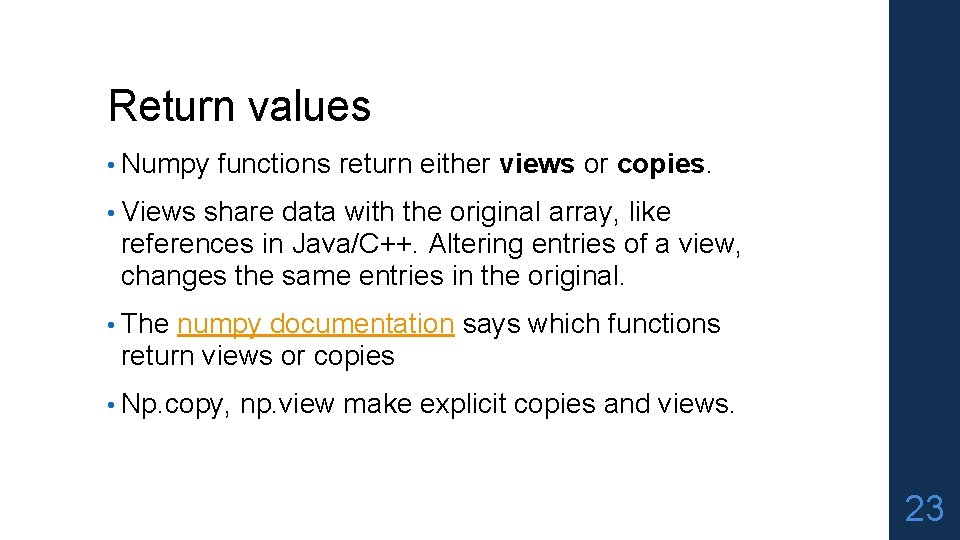
Return values • Numpy functions return either views or copies. • Views share data with the original array, like references in Java/C++. Altering entries of a view, changes the same entries in the original. • The numpy documentation says which functions return views or copies • Np. copy, np. view make explicit copies and views. 23

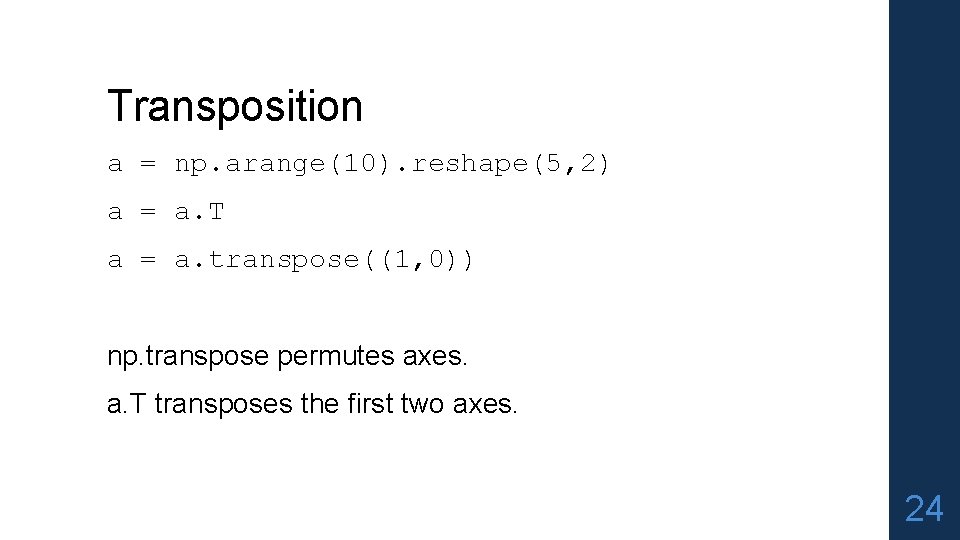
Transposition a = np. arange(10). reshape(5, 2) a = a. T a = a. transpose((1, 0)) np. transpose permutes axes. a. T transposes the first two axes. 24

Saving and loading arrays np. savez(‘data. npz’, a=a) data = np. load(‘data. npz’) a = data[‘a’] 1. NPZ files can hold multiple arrays 2. np. savez_compressed similar. 25

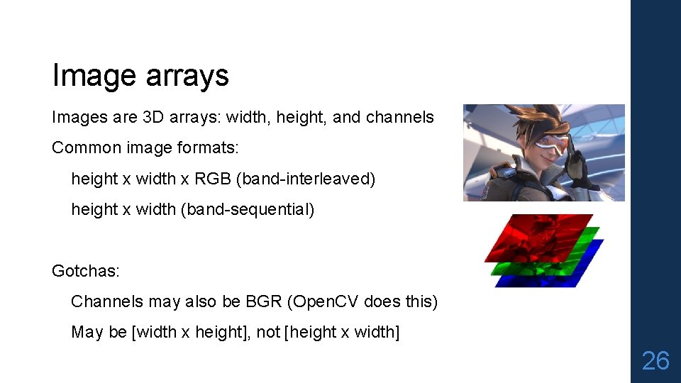
Image arrays Images are 3 D arrays: width, height, and channels Common image formats: height x width x RGB (band-interleaved) height x width (band-sequential) Gotchas: Channels may also be BGR (Open. CV does this) May be [width x height], not [height x width] 26

Saving and Loading Images Sci. Py: skimage. io. imread, skimage. io. imsave height x width x RGB PIL / Pillow: PIL. Image. open, Image. save width x height x RGB Open. CV: cv 2. imread, cv 2. imwrite height x width x BGR 27

Recap We just saw how to create arrays, reshape them, and permute axes Questions so far? 28

Recap We just saw how to create arrays, reshape them, and permute axes Questions so far? Now: let’s do some math 29

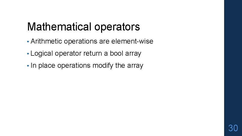
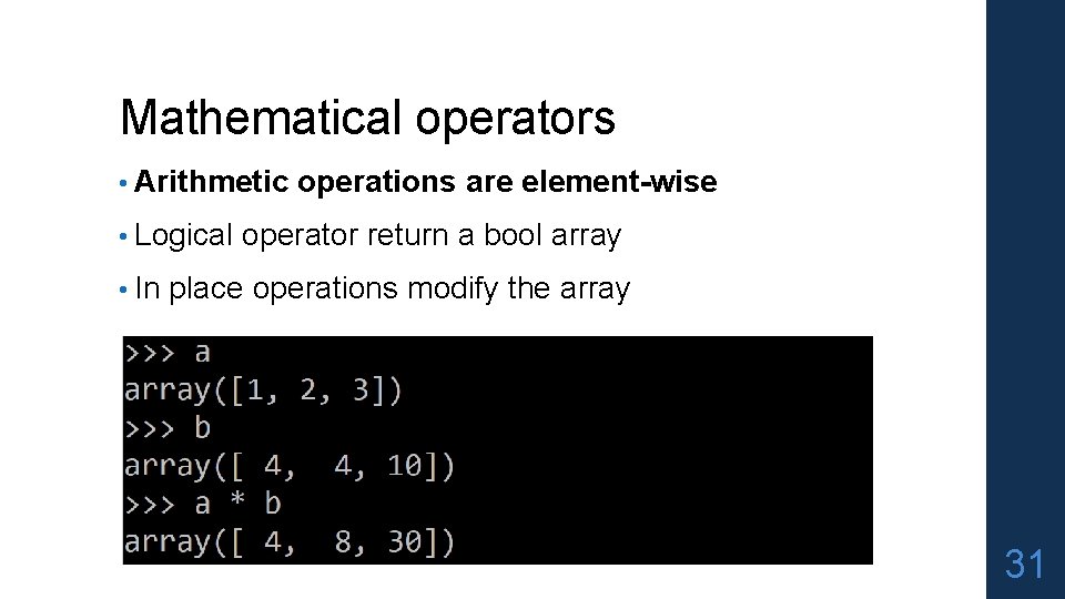
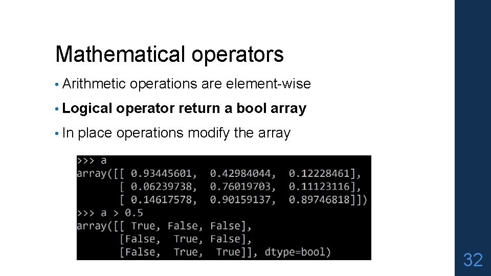
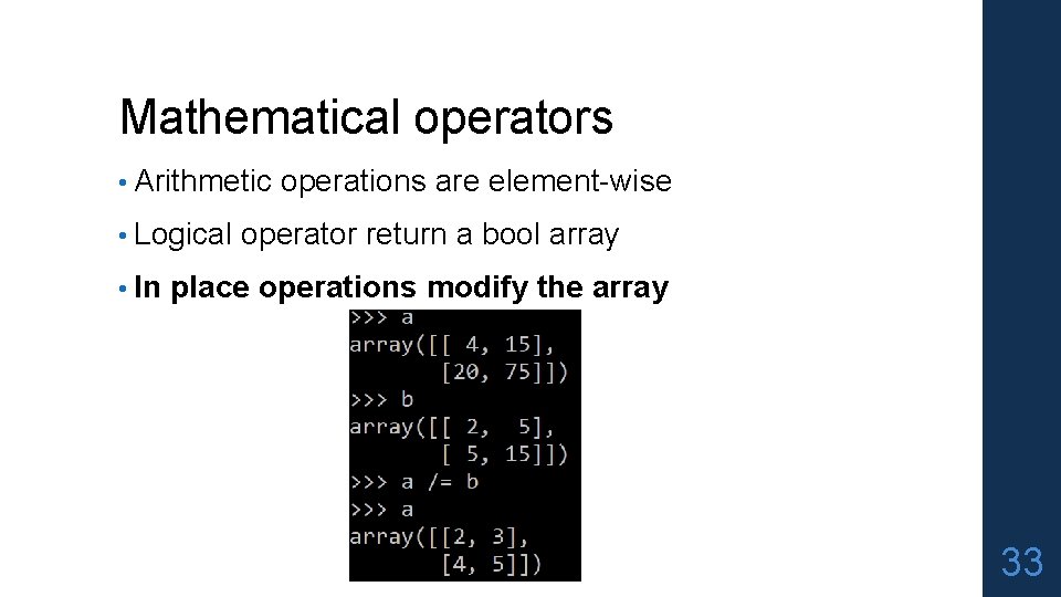
Mathematical operators • Arithmetic operations are element-wise • Logical operator return a bool array • In place operations modify the array 30

Mathematical operators • Arithmetic operations are element-wise • Logical operator return a bool array • In place operations modify the array 31

Mathematical operators • Arithmetic operations are element-wise • Logical operator return a bool array • In place operations modify the array 32

Mathematical operators • Arithmetic operations are element-wise • Logical operator return a bool array • In place operations modify the array 33

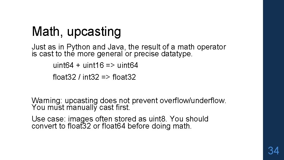
Math, upcasting Just as in Python and Java, the result of a math operator is cast to the more general or precise datatype. uint 64 + uint 16 => uint 64 float 32 / int 32 => float 32 Warning: upcasting does not prevent overflow/underflow. You must manually cast first. Use case: images often stored as uint 8. You should convert to float 32 or float 64 before doing math. 34

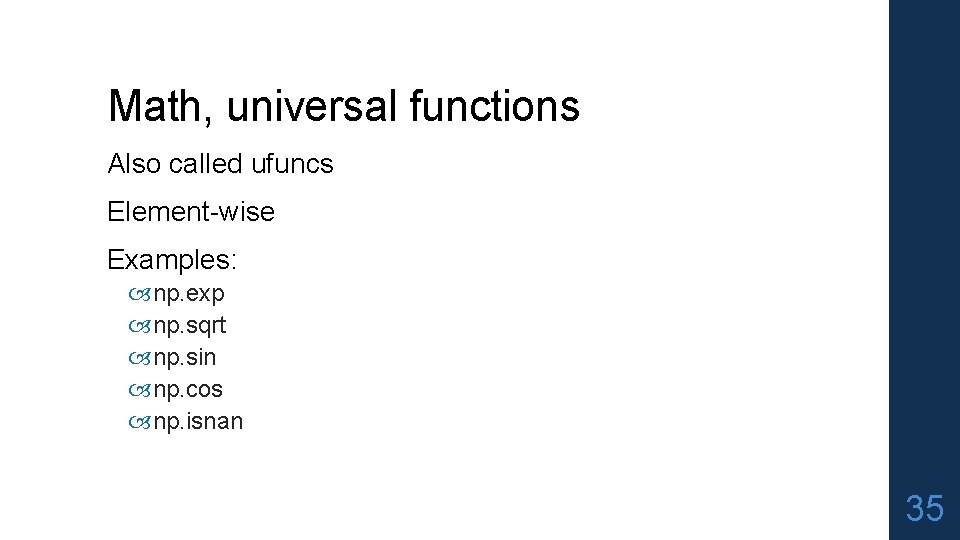
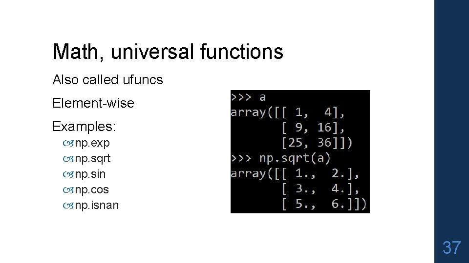
Math, universal functions Also called ufuncs Element-wise Examples: np. exp np. sqrt np. sin np. cos np. isnan 35

Math, universal functions Also called ufuncs Element-wise Examples: np. exp np. sqrt np. sin np. cos np. isnan 36

Math, universal functions Also called ufuncs Element-wise Examples: np. exp np. sqrt np. sin np. cos np. isnan 37

Indexing x[0, 0] # top-left element x[0, -1] # first row, last column x[0, : ] # first row (many entries) x[: , 0] # first column (many entries) Notes: Zero-indexing Multi-dimensional indices are comma-separated (i. e. , a tuple) 38

Indexing, slices and arrays I[1: -1, 1: -1] # select all but one-pixel border I = I[: , : : -1] # swap channel order I[I<10] = 0 # set dark pixels to black I[[1, 3], : ] # select 2 nd and 4 th row 1. Slices are views. Writing to a slice overwrites the original array. 2. Can also index by a list or boolean array. 39

Python Slicing Syntax: start: stop: step a = list(range(10)) a[: 3] # indices 0, 1, 2 a[-3: ] # indices 7, 8, 9 a[3: 8: 2] # indices 3, 5, 7 a[4: 1: -1] # indices 4, 3, 2 (this one is tricky) 40

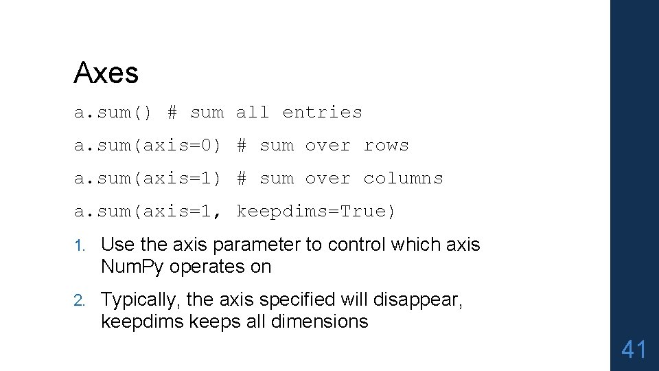
Axes a. sum() # sum all entries a. sum(axis=0) # sum over rows a. sum(axis=1) # sum over columns a. sum(axis=1, keepdims=True) 1. Use the axis parameter to control which axis Num. Py operates on 2. Typically, the axis specified will disappear, keepdims keeps all dimensions 41

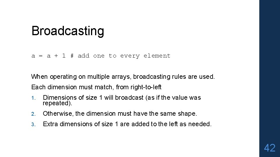
Broadcasting a = a + 1 # add one to every element When operating on multiple arrays, broadcasting rules are used. Each dimension must match, from right-to-left 1. Dimensions of size 1 will broadcast (as if the value was repeated). 2. Otherwise, the dimension must have the same shape. 3. Extra dimensions of size 1 are added to the left as needed. 42

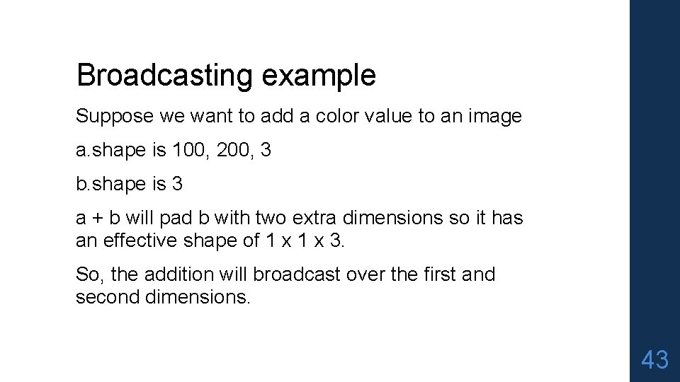
Broadcasting example Suppose we want to add a color value to an image a. shape is 100, 200, 3 b. shape is 3 a + b will pad b with two extra dimensions so it has an effective shape of 1 x 3. So, the addition will broadcast over the first and second dimensions. 43

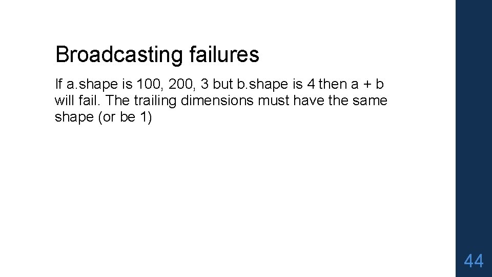
Broadcasting failures If a. shape is 100, 200, 3 but b. shape is 4 then a + b will fail. The trailing dimensions must have the same shape (or be 1) 44

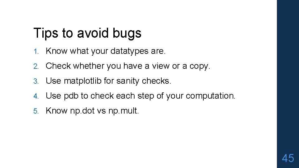
Tips to avoid bugs 1. Know what your datatypes are. 2. Check whether you have a view or a copy. 3. Use matplotlib for sanity checks. 4. Use pdb to check each step of your computation. 5. Know np. dot vs np. mult. 45

Average images Who is this? 46

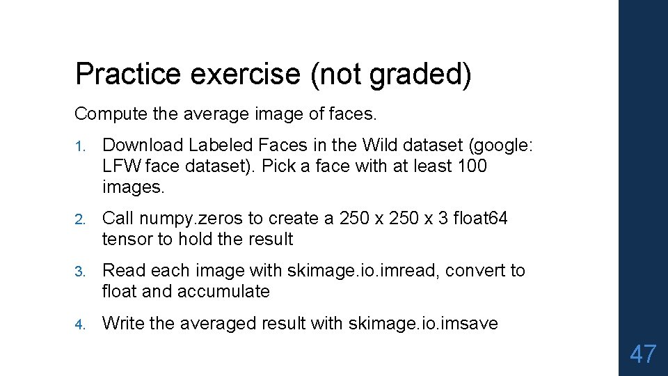
Practice exercise (not graded) Compute the average image of faces. 1. Download Labeled Faces in the Wild dataset (google: LFW face dataset). Pick a face with at least 100 images. 2. Call numpy. zeros to create a 250 x 3 float 64 tensor to hold the result 3. Read each image with skimage. io. imread, convert to float and accumulate 4. Write the averaged result with skimage. io. imsave 47