ANKARA UNIVERSITY DEPARTMENT OF ENERGY ENGINEERING NUMERICAL METHODS

ANKARA UNIVERSITY DEPARTMENT OF ENERGY ENGINEERING NUMERICAL METHODS INSTRUCTOR DR. ÖZGÜR SELİMOĞLU

CONTENTS ➢ Interpolations and Curve Fitting c) Least-Squares Fit

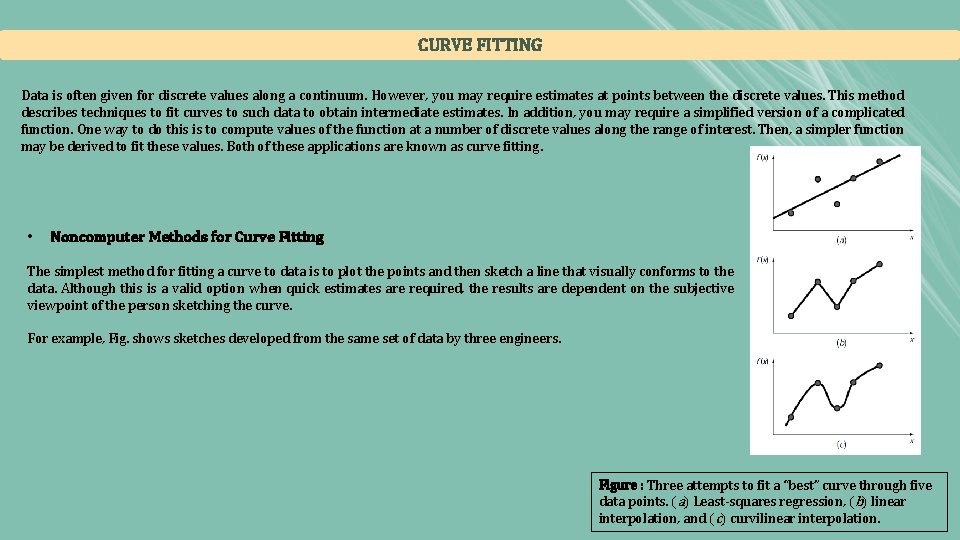
CURVE FITTING Data is often given for discrete values along a continuum. However, you may require estimates at points between the discrete values. This method describes techniques to fit curves to such data to obtain intermediate estimates. In addition, you may require a simplified version of a complicated function. One way to do this is to compute values of the function at a number of discrete values along the range of interest. Then, a simpler function may be derived to fit these values. Both of these applications are known as curve fitting. • Noncomputer Methods for Curve Fitting The simplest method for fitting a curve to data is to plot the points and then sketch a line that visually conforms to the data. Although this is a valid option when quick estimates are required, the results are dependent on the subjective viewpoint of the person sketching the curve. For example, Fig. shows sketches developed from the same set of data by three engineers. Figure : Three attempts to fit a “best” curve through five data points. (a) Least-squares regression, (b) linear interpolation, and (c) curvilinear interpolation.

INTERPOLATIONS AND CURVE FITTING

INTERPOLATIONS AND CURVE FITTING

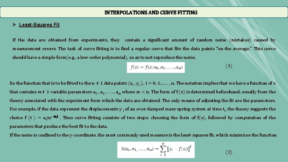
INTERPOLATIONS AND CURVE FITTING Ø Least-Squares Fit If the data are obtained from experiments, they contain a significant amount of random noise (mistakes) caused by measurement errors. The task of curve fitting is to find a regular curve that fits the data points “on the average. ” This curve should have a simple form(e. g. , a low-order polynomial), so as to not reproduce the noise. (1) Be the function that is to be fitted to the n + 1 data points (xi , yi ), i = 0, 1, . . , n. The notation implies that we have a function of x that contains m+ 1 variable parameters a 0 , a 1 , . . . , am where m < n. The form of f (x) is determined beforehand, usually from theory associated with the experiment from which the data are obtained. The only means of adjusting the fit are the parameters. For example, if the data represent the displacements y i of an over-damped mass-spring system at time ti, theory suggests the choice f (t ) = a 0 te−a 1 t. Thus curve fitting consists of two steps: choosing the form of f(x), followed by computation of the parameters that produce the best fit to the data. If the noise is confined to the y-coordinate, the most commonly used measure is the least-squares fit, which minimizes the function (2)

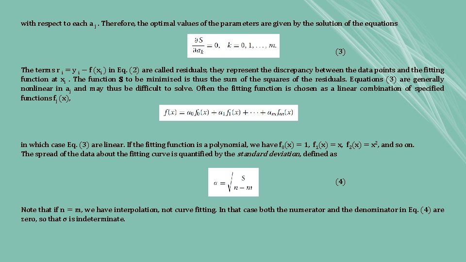
with respect to each a j. Therefore, the optimal values of the parameters are given by the solution of the equations (3) The terms r i = y i − f (xi ) in Eq. (2) are called residuals; they represent the discrepancy between the data points and the fitting function at xi. The function S to be minimized is thus the sum of the squares of the residuals. Equations (3) are generally nonlinear in aj and may thus be difficult to solve. Often the fitting function is chosen as a linear combination of specified functions fj (x), in which case Eq. (3) are linear. If the fitting function is a polynomial, we have f 0(x) = 1, f 1(x) = x, f 2(x) = x 2, and so on. The spread of the data about the fitting curve is quantified by the standard deviation, defined as (4) Note that if n = m, we have interpolation, not curve fitting. In that case both the numerator and the denominator in Eq. (4) are zero, so that σ is indeterminate.

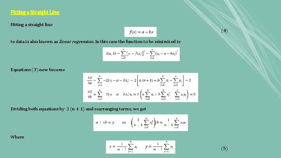
Fitting a Straight Line Fitting a straight line (4) to data is also known as linear regression. In this case the function to be minimized is Equations (3) now become Dividing both equations by 2 (n + 1) and rearranging terms, we get Where (5)

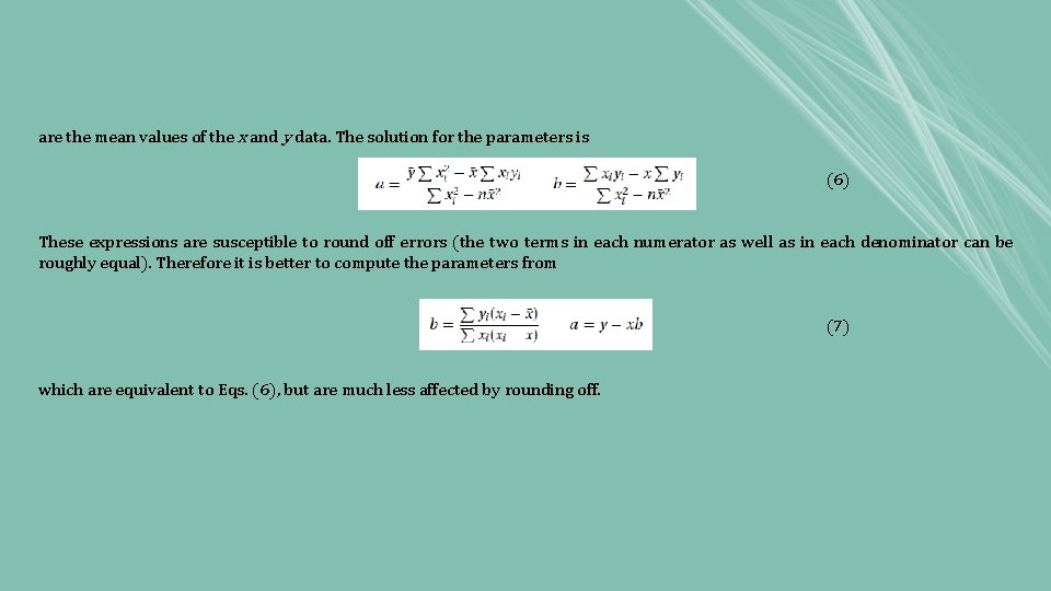
are the mean values of the x and y data. The solution for the parameters is (6) These expressions are susceptible to round off errors (the two terms in each numerator as well as in each denominator can be roughly equal). Therefore it is better to compute the parameters from (7) which are equivalent to Eqs. (6), but are much less affected by rounding off.

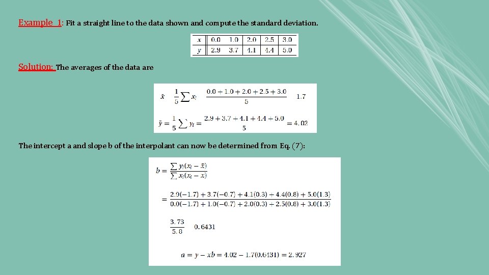
Example 1: Fit a straight line to the data shown and compute the standard deviation. Solution: The averages of the data are The intercept a and slope b of the interpolant can now be determined from Eq. (7):

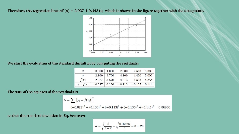
Therefore, the regression line is f (x) = 2. 927 + 0. 6431 x, which is shown in the figure together with the data points. We start the evaluation of the standard deviation by computing the residuals: The sum of the squares of the residuals is so that the standard deviation in Eq. becomes

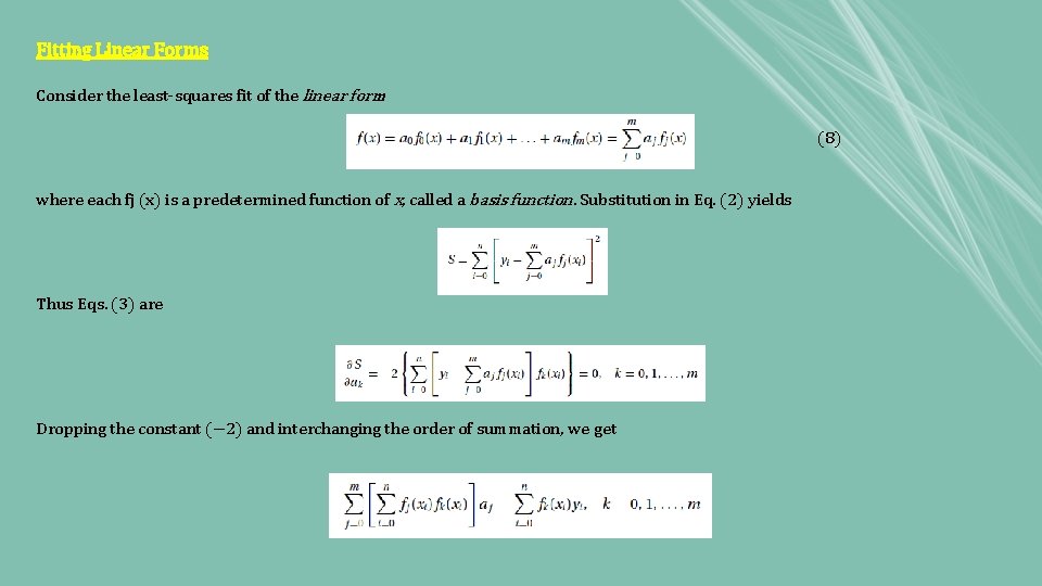
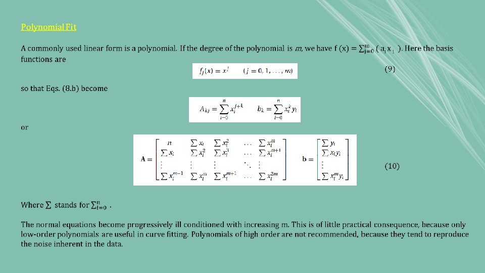
Fitting Linear Forms Consider the least-squares fit of the linear form (8) where each fj (x) is a predetermined function of x, called a basis function. Substitution in Eq. (2) yields Thus Eqs. (3) are Dropping the constant (− 2) and interchanging the order of summation, we get

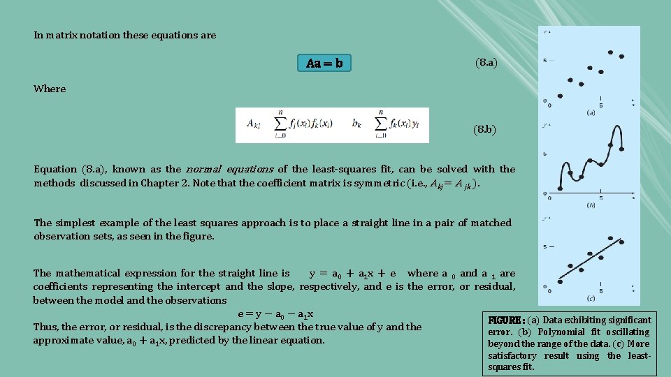
In matrix notation these equations are Aa = b (8. a) Where (8. b) Equation (8. a), known as the normal equations of the least-squares fit, can be solved with the methods discussed in Chapter 2. Note that the coefficient matrix is symmetric (i. e. , Akj = A jk ). The simplest example of the least squares approach is to place a straight line in a pair of matched observation sets, as seen in the figure. The mathematical expression for the straight line is y = a 0 + a 1 x + e where a 0 and a 1 are coefficients representing the intercept and the slope, respectively, and e is the error, or residual, between the model and the observations e = y − a 0 − a 1 x FIGURE : (a) Data exhibiting significant Thus, the error, or residual, is the discrepancy between the true value of y and the error. (b) Polynomial fit oscillating approximate value, a 0 + a 1 x, predicted by the linear equation. beyond the range of the data. (c) More satisfactory result using the leastsquares fit.

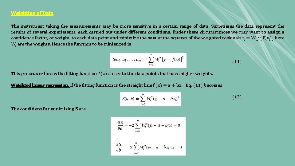
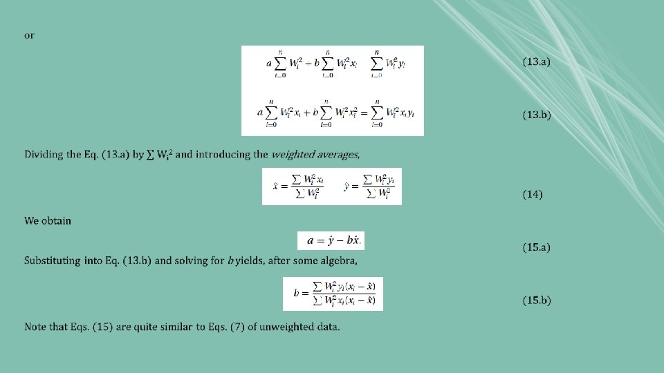
Weighting of Data The instrument taking the measurements may be more sensitive in a certain range of data. Sometimes the data represent the results of several experiments, each carried out under different conditions. Under these circumstances we may want to assign a confidence factor, or weight, to each data point and minimize the sum of the squares of the weighted residuals ri = Wi[yi-f(xi)] here Wi are the weights. Hence the function to be minimized is (11) This procedure forces the fitting function f (x) closer to the data points that have higher weights. Weighted linear regression. If the fitting function is the straight line f (x) = a + bx, Eq. (11) becomes (12) The conditions for minimizing S are

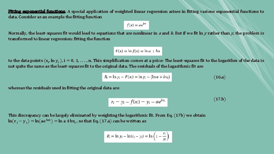
Fitting exponential functions. A special application of weighted linear regression arises in fitting various exponential functions to data. Consider as an example the fitting function Normally, the least-squares fit would lead to equations that are nonlinear in a and b. But if we fit ln y rather than y, the problem is transformed to linear regression: fitting the function to the data points (xi, ln yi ), i = 0, 1, . . . , n. This simplification comes at a price: The least-squares fit to the logarithm of the data is not quite the same as the least-squares fit to the original data. The residuals of the logarithmic fit are (16. a) whereas the residuals used in fitting the original data are (17. b) This discrepancy can be largely eliminated by weighting the logarithmic fit. From Eq. (17 b) we obtain ln(r i − y i ) = ln(ae bxi ) = ln a +bxi , so that Eq. (17. a) can be written as

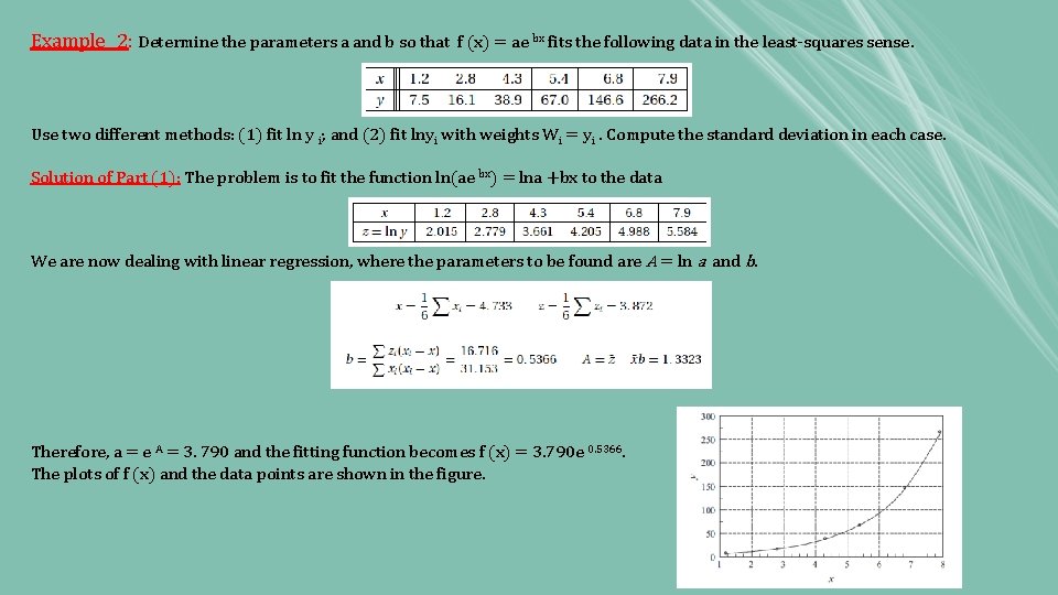
Example 2: Determine the parameters a and b so that f (x) = ae bx fits the following data in the least-squares sense. Use two different methods: (1) fit ln y i; and (2) fit lnyi with weights Wi = yi. Compute the standard deviation in each case. Solution of Part (1): The problem is to fit the function ln(ae bx) = lna +bx to the data We are now dealing with linear regression, where the parameters to be found are A = ln a and b. Therefore, a = e A = 3. 790 and the fitting function becomes f (x) = 3. 790 e 0. 5366. The plots of f (x) and the data points are shown in the figure.

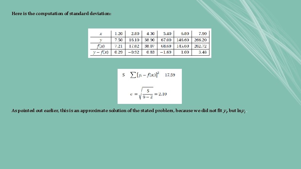
Here is the computation of standard deviation: As pointed out earlier, this is an approximate solution of the stated problem, because we did not fit yi, but lnyi.

Solution of Part (2): We again fit ln(ae bx) = lna +bx to z = ln y, but this time using the weights Wi = yi. From Eqs. (3. 27) the weighted averages of the data are (recall that we fit z = ln y) and Eqs. yield for the parameters Therefore, so that the fitting function is f (x) = 3. 622 e 0. 5440 x. As expected, this result is somewhat different from that obtained in Part (1).

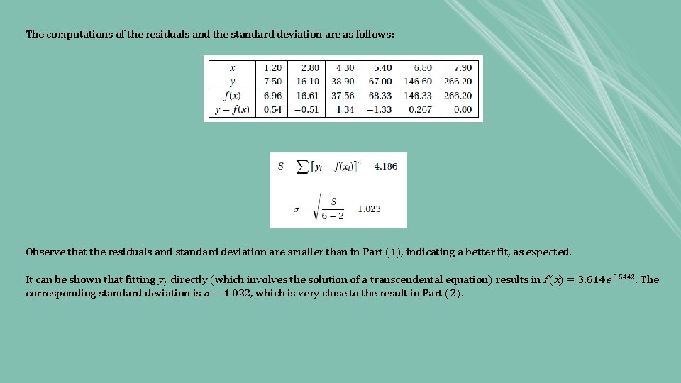
The computations of the residuals and the standard deviation are as follows: Observe that the residuals and standard deviation are smaller than in Part (1), indicating a better fit, as expected. It can be shown that fitting yi directly (which involves the solution of a transcendental equation) results in f (x) = 3. 614 e 0. 5442. The corresponding standard deviation is σ = 1. 022, which is very close to the result in Part (2).

REFERENCES • Jaan Kiusalaas, “Numerical Methods in Engineering with Python 3”, 3 rd Edition, Cambridge, NY, 2013