Interpolation A method of constructing a function that

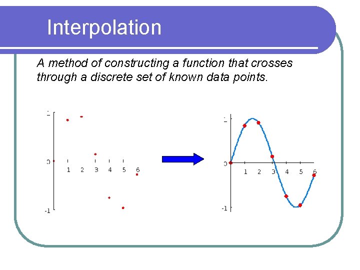
Interpolation A method of constructing a function that crosses through a discrete set of known data points. .

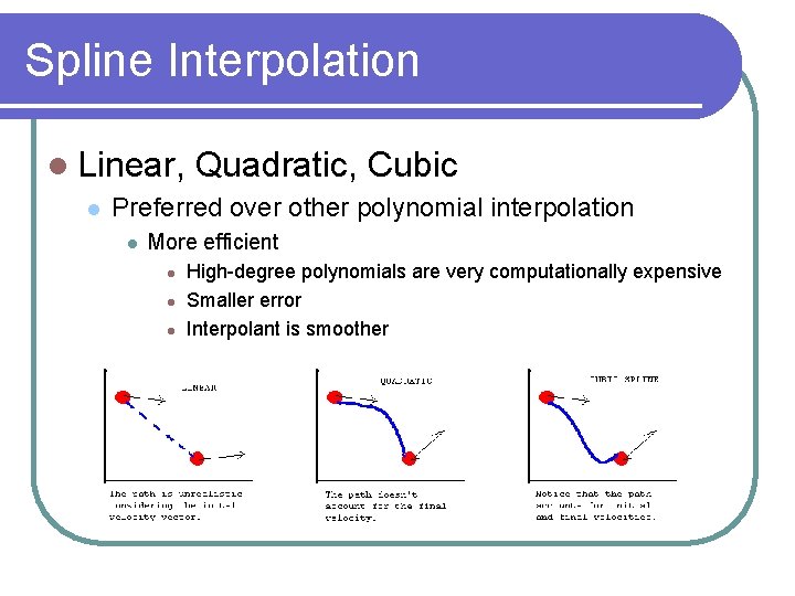
Spline Interpolation Linear, Quadratic, Cubic Preferred over other polynomial interpolation More efficient High-degree polynomials are very computationally expensive Smaller error Interpolant is smoother

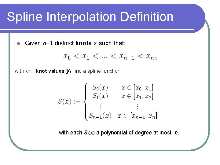
Spline Interpolation Definition Given n+1 distinct knots xi such that: with n+1 knot values yi find a spline function with each Si(x) a polynomial of degree at most n.

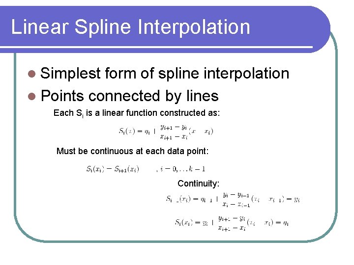
Linear Spline Interpolation Simplest form of spline interpolation Points connected by lines Each Si is a linear function constructed as: Must be continuous at each data point: Continuity:

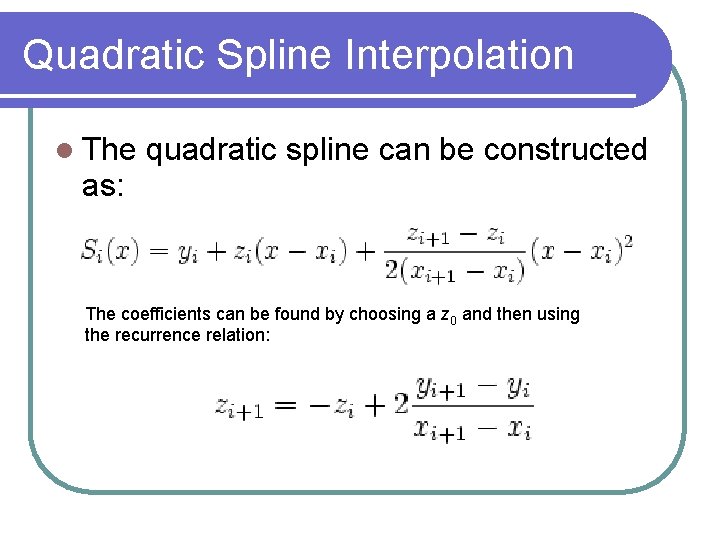
Quadratic Spline Interpolation The quadratic spline can be constructed as: The coefficients can be found by choosing a z 0 and then using the recurrence relation:

Quadratic Splines 2 Quadratic splines are rarely used for interpolation for practical purposes Ideally quadratic splines are only used to understand cubic splines

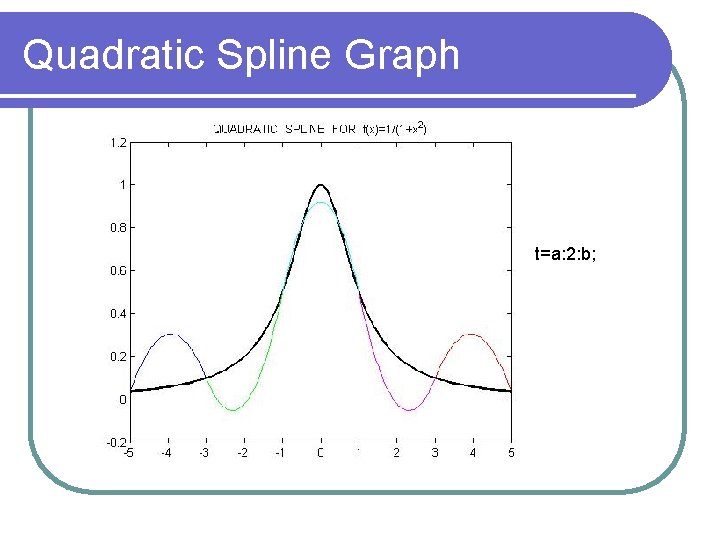
Quadratic Spline Graph t=a: 2: b;

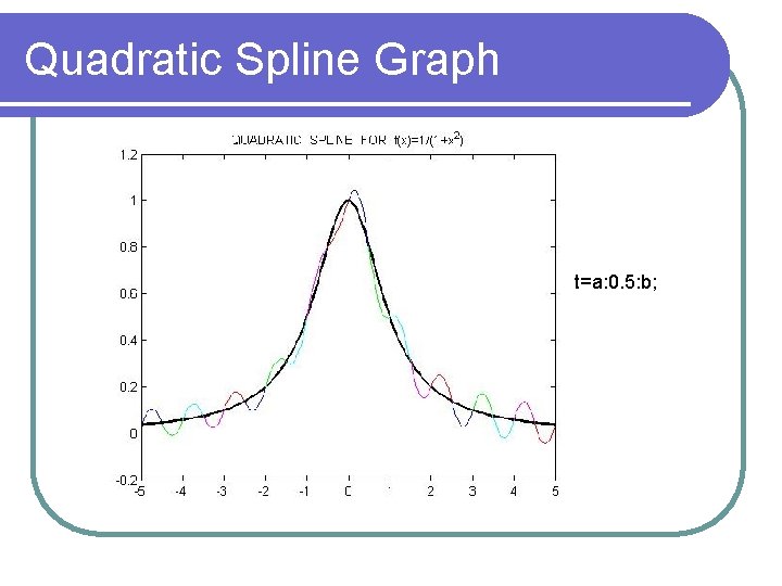
Quadratic Spline Graph t=a: 0. 5: b;

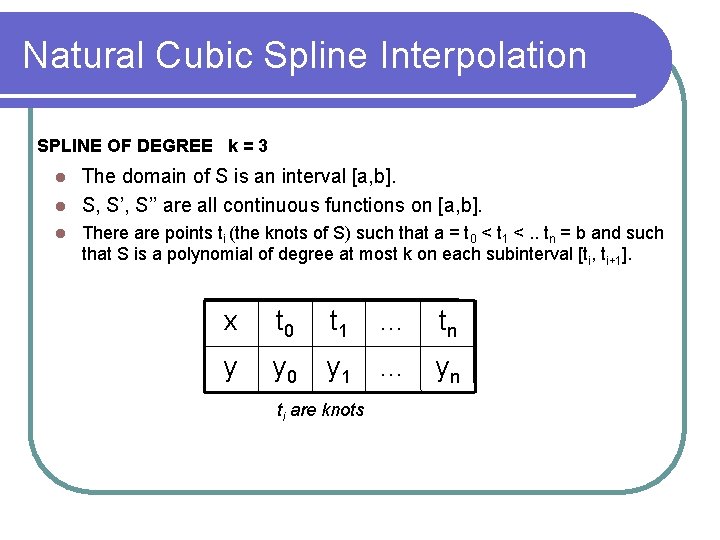
Natural Cubic Spline Interpolation SPLINE OF DEGREE k = 3 The domain of S is an interval [a, b]. S, S’’ are all continuous functions on [a, b]. There are points ti (the knots of S) such that a = t 0 < t 1 <. . tn = b and such that S is a polynomial of degree at most k on each subinterval [ti, ti+1]. x t 0 t 1 … tn y y 0 y 1 … yn ti are knots

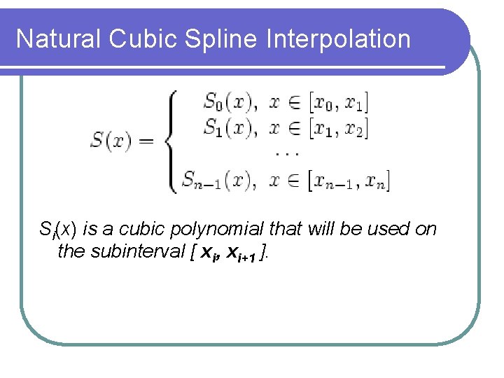
Natural Cubic Spline Interpolation Si(x) is a cubic polynomial that will be used on the subinterval [ xi, xi+1 ].

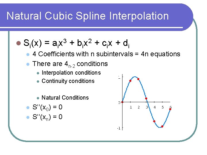
Natural Cubic Spline Interpolation Si(x) 4 Coefficients with n subintervals = 4 n equations There are 4 n-2 conditions Interpolation conditions Continuity conditions Natural Conditions = aix 3 + bix 2 + cix + di S’’(x 0) = 0 S’’(xn) = 0

Natural Cubic Spline Interpolation Algorithm Define Zi = S’’(ti) On each [ti, ti+1] S’’ is a linear polynomial with Si’’(ti) = zi, Si’’ (ti+1) = z+1 Then Where hi = ti+1 – ti Integrating twice yields:

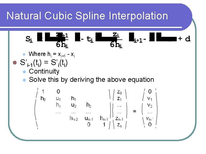
Natural Cubic Spline Interpolation Where hi = xi+1 - xi S’i-1(ti) = S’i(ti) Continuity Solve this by deriving the above equation

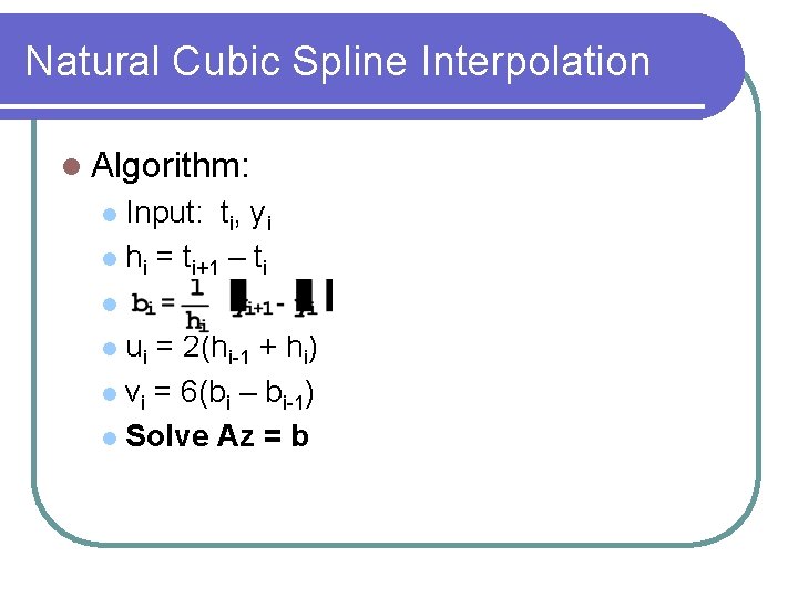
Natural Cubic Spline Interpolation Algorithm: Input: ti, yi hi = ti+1 – ti a ui = 2(hi-1 + hi) vi = 6(bi – bi-1) Solve Az = b

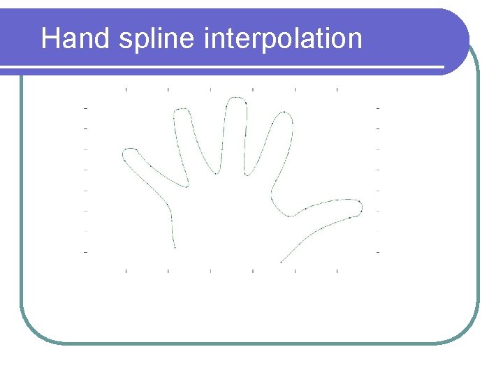
Hand spline interpolation

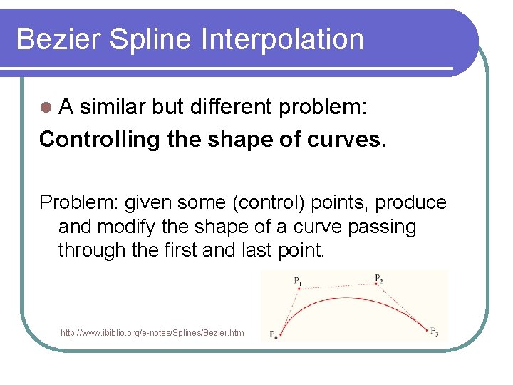
Bezier Spline Interpolation A similar but different problem: Controlling the shape of curves. Problem: given some (control) points, produce and modify the shape of a curve passing through the first and last point. http: //www. ibiblio. org/e-notes/Splines/Bezier. htm

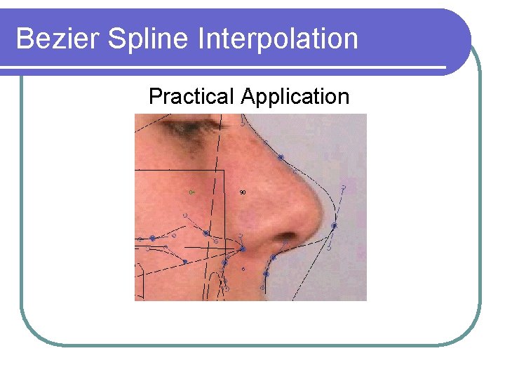
Bezier Spline Interpolation Practical Application

Bezier Spline Interpolation Idea: Build functions that are combinations of some basic and simpler functions. Basic functions: B-splines Bernstein polynomials

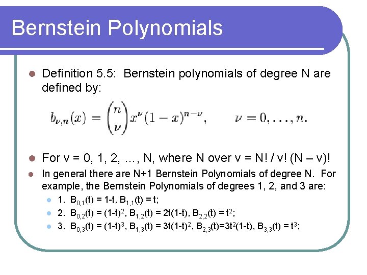
Bernstein Polynomials Definition 5. 5: Bernstein polynomials of degree N are defined by: For v = 0, 1, 2, …, N, where N over v = N! / v! (N – v)! In general there are N+1 Bernstein Polynomials of degree N. For example, the Bernstein Polynomials of degrees 1, 2, and 3 are: 1. B 0, 1(t) = 1 -t, B 1, 1(t) = t; 2. B 0, 2(t) = (1 -t)2, B 1, 2(t) = 2 t(1 -t), B 2, 2(t) = t 2; 3. B 0, 3(t) = (1 -t)3, B 1, 3(t) = 3 t(1 -t)2, B 2, 3(t)=3 t 2(1 -t), B 3, 3(t) = t 3;

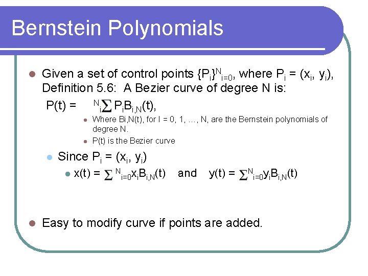
Bernstein Polynomials Given a set of control points {Pi}Ni=0, where Pi = (xi, yi), Definition 5. 6: A Bezier curve of degree N is: P(t) = Ni=0 Pi. Bi, N(t), Since Pi = (xi, yi) Where Bi, N(t), for I = 0, 1, …, N, are the Bernstein polynomials of degree N. P(t) is the Bezier curve x(t) = N i=0 xi. Bi, N(t) and y(t) = N i=0 yi. Bi, N(t) Easy to modify curve if points are added.

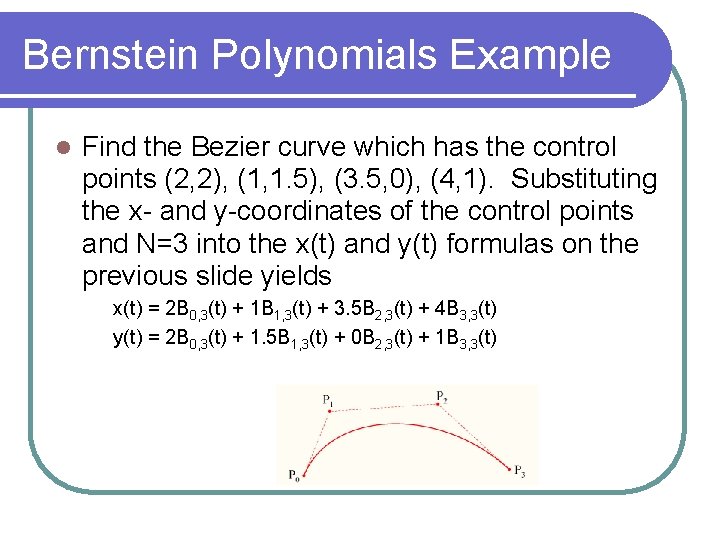
Bernstein Polynomials Example Find the Bezier curve which has the control points (2, 2), (1, 1. 5), (3. 5, 0), (4, 1). Substituting the x- and y-coordinates of the control points and N=3 into the x(t) and y(t) formulas on the previous slide yields x(t) = 2 B 0, 3(t) + 1 B 1, 3(t) + 3. 5 B 2, 3(t) + 4 B 3, 3(t) y(t) = 2 B 0, 3(t) + 1. 5 B 1, 3(t) + 0 B 2, 3(t) + 1 B 3, 3(t)