Spatial Analysis Geostatistics Methods of Interpolation Linear interpolation

Spatial Analysis & Geostatistics Methods of Interpolation Linear interpolation using an equation to compute z at any point on a triangle

Linear Interpolation

Clough-Tocher Interpolation – Using cubic polynomial defined by 12 parameters

Inverse Distance Weighted Interpolation – nodal function constants

Inverse Distance Weighted Interpolation –gradient method

Inverse Distance Weighted Interpolation –cubic method

Inverse Distance Weighted Interpolation –cubic method - truncated

Natural Neighbor Interpolation

Kriging

Differences between kriging and nn

More formal definition of kriging Kriging is based on the assumption that the parameter being interpolated can be treated as a regionalized variable. A regionalized variable is intermediate between a truly random variable and a completely deterministic variable in that it varies in a continuous manner from one location to the next and therefore points that are near each other have a certain degree of spatial correlation, but points that are widely separated are statistically independent (Davis, 1986). Kriging is a set of linear regression routines which minimize estimation variance from a predefined covariance model. Once the experimental variogram is computed, the next step is to define a model variogram. A model variogram is a simple mathematical function that models the trend in the experimental variogram

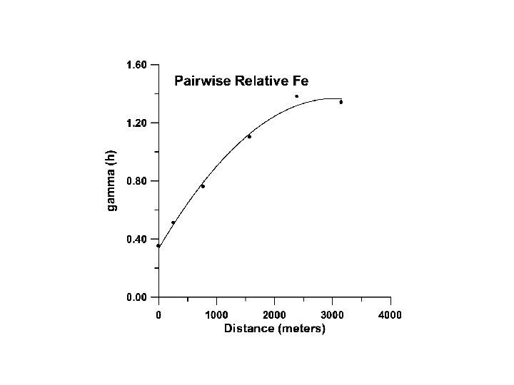
The first step in ordinary kriging is to construct a variogram from the scatter point set to be interpolated. A variogram consists of two parts: an experimental variogram and a model variogram. Suppose that the value to be interpolated is referred to as f. The experimental variogram is found by calculating the variance (g) of each point in the set with respect to each of the other points and plotting the variances versus distance (h) between the points. Several formulas can be used to compute the variance, but it is typically computed as one half the difference in f squared.

Normal Score Transform of the Pu Isotopic Ratio into Y value. Variogram Modeling of the Normal Score Values Y Using Trial & Error Approach to Fit a Model. Construction of a ccdf Using the Pu Isotopic Ratios. Stochastic Simulation Techniques Bivariate Normality Test If Normal Proceed with s. Gs. If Normal Assumption Violated Select Other Simulation Routines Define Random Path that visits Each Grid Node Once. Specified Number of Neighboring Conditioning Data Including Original Data and Previously Simulated Values. Use SK with the Above Variogram Model to Determine the Parameters of the ccdf of the Y Variable at Location (u). Draw a Simulated Value y(l)(u) from that ccdf and Add this Value to the Data Set. Proceed to the Next Node and Loop Until all Nodes Are Simulated. One Hundred Realizations Were Conducted. Setting A Different Random Path For Each Realization. Backtransformed the Simulated Normal Values {y(l)(u), u A} into Simulated Values of the Original Variable z. Where l represents realization, u location, and A the study area.

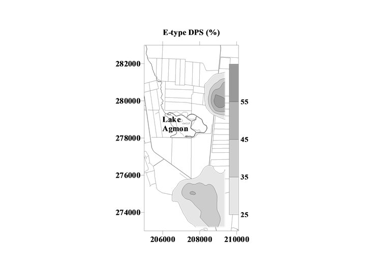
Probability of Exceedance

The level of variation present in all scales can be described by a single parameter, the fractal dimension D, defined by Mandelbrat, (1982): where N is the number of steps used to measure a pattern unit length and r is the scale ratio. In practice, we estimated the D values from the following relationships: where h is the sampling interval and (h) is the spatial structure. By plotting log (h) versus log(h), the slope of the line is equal to 4 – 2 D

Attribute D Lag (m) Elevation 50 1. 2 Mean Snow Depth 50 1. 4 Organic C 35 1. 7 p. H 35 1. 7 Bulk density 50 1. 8 Soil Moisture Content 50 1. 7 L* 35 1. 6 a* 35 1. 7 b* 35 1. 7