Image Interpolation Introduction What is image interpolation Why

Image Interpolation • Introduction – What is image interpolation? – Why do we need it? • Interpolation Techniques – 1 D zero-order, first-order, third-order – 2 D zero-order, first-order, third-order – Directional interpolation* • Interpolation Applications – Digital zooming (resolution enhancement) – Image inpainting (error concealment) – Geometric transformations EE 465: Introduction to Digital Image Processing 1

Introduction • What is image interpolation? – An image f(x, y) tells us the intensity values at the integral lattice locations, i. e. , when x and y are both integers – Image interpolation refers to the “guess” of intensity values at missing locations, i. e. , x and y can be arbitrary – Note that it is just a guess (Note that all sensors have finite sampling distance) EE 465: Introduction to Digital Image Processing 2

Introduction (Con’t) • Why do we need image interpolation? – We want BIG images • When we see a video clip on a PC, we like to see it in the full screen mode – We want GOOD images • If some block of an image gets damaged during the transmission, we want to repair it – We want COOL images • Manipulate images digitally can render fancy artistic effects as we often see in movies EE 465: Introduction to Digital Image Processing 3

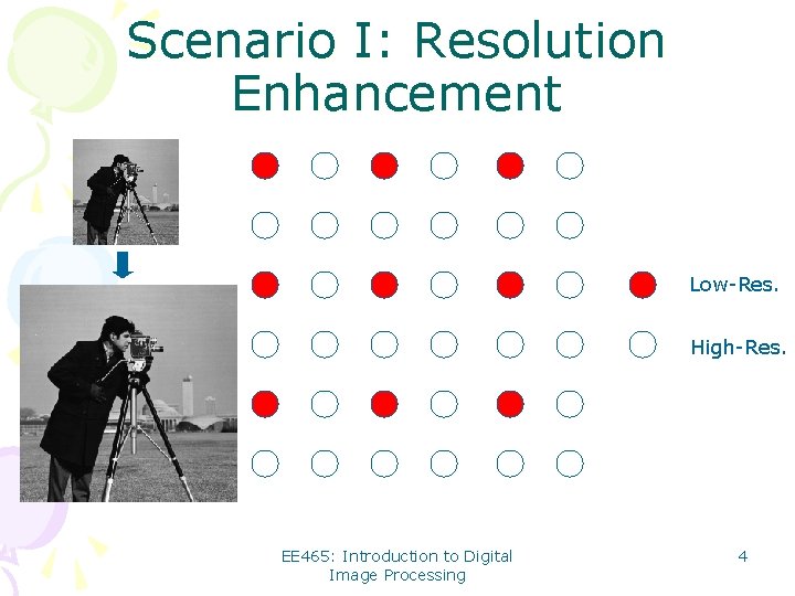
Scenario I: Resolution Enhancement Low-Res. High-Res. EE 465: Introduction to Digital Image Processing 4

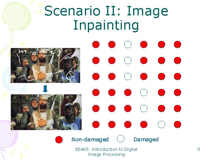
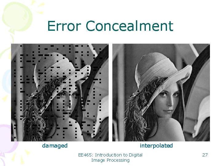
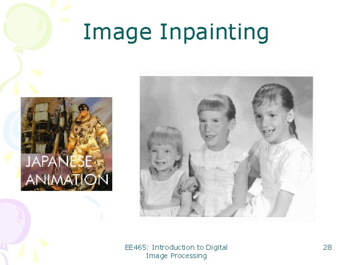
Scenario II: Image Inpainting Non-damaged Damaged EE 465: Introduction to Digital Image Processing 5

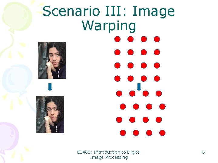
Scenario III: Image Warping EE 465: Introduction to Digital Image Processing 6

Image Interpolation • Introduction – What is image interpolation? – Why do we need it? • Interpolation Techniques – 1 D zero-order, first-order, third-order – 2 D zero-order, first-order, third-order – Directional interpolation* • Interpolation Applications – Digital zooming (resolution enhancement) – Image inpainting (error concealment) – Geometric transformations EE 465: Introduction to Digital Image Processing 7

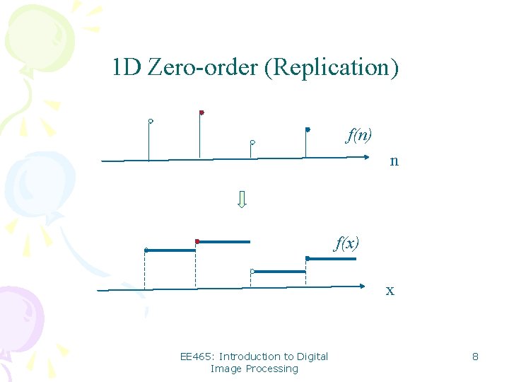
1 D Zero-order (Replication) f(n) n f(x) x EE 465: Introduction to Digital Image Processing 8

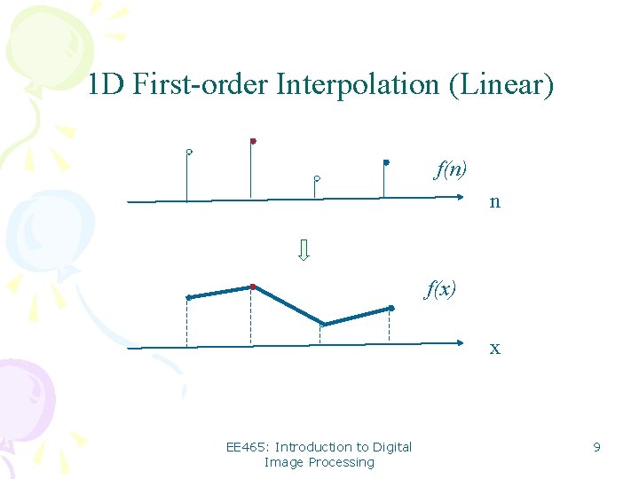
1 D First-order Interpolation (Linear) f(n) n f(x) x EE 465: Introduction to Digital Image Processing 9

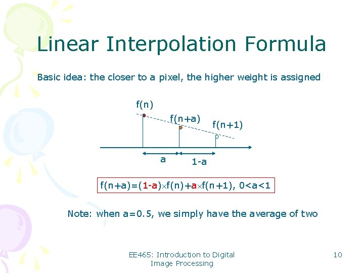
Linear Interpolation Formula Basic idea: the closer to a pixel, the higher weight is assigned f(n) f(n+a) a f(n+1) 1 -a f(n+a)=(1 -a) f(n)+a f(n+1), 0<a<1 Note: when a=0. 5, we simply have the average of two EE 465: Introduction to Digital Image Processing 10

Numerical Examples f(n)=[0, 120, 180, 120, 0] Interpolate at 1/2 -pixel f(x)=[0, 60, 120, 150, 180, 150, 120, 60, 0], x=n/2 Interpolate at 1/3 -pixel f(x)=[0, 20, 40, 60, 80, 100, 120, 130, 140, 150, 160, 170, 180, …], x=n/6 EE 465: Introduction to Digital Image Processing 11

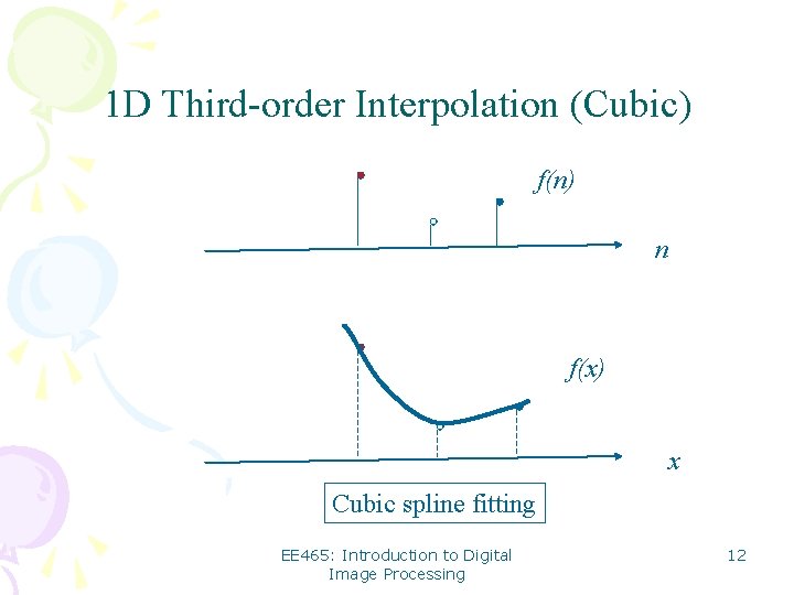
1 D Third-order Interpolation (Cubic) f(n) n f(x) x Cubic spline fitting EE 465: Introduction to Digital Image Processing 12

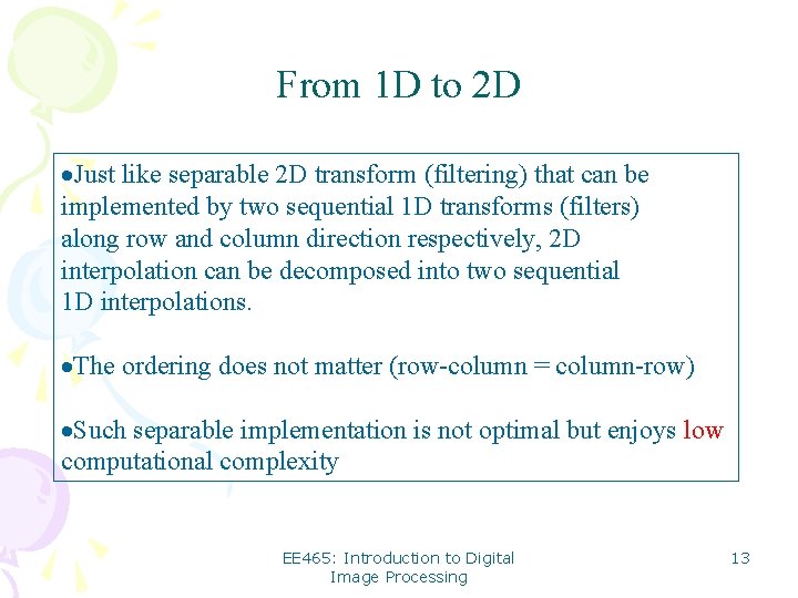
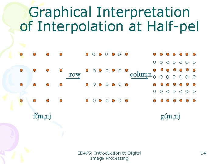
From 1 D to 2 D ·Just like separable 2 D transform (filtering) that can be implemented by two sequential 1 D transforms (filters) along row and column direction respectively, 2 D interpolation can be decomposed into two sequential 1 D interpolations. ·The ordering does not matter (row-column = column-row) ·Such separable implementation is not optimal but enjoys low computational complexity EE 465: Introduction to Digital Image Processing 13

Graphical Interpretation of Interpolation at Half-pel row column f(m, n) g(m, n) EE 465: Introduction to Digital Image Processing 14

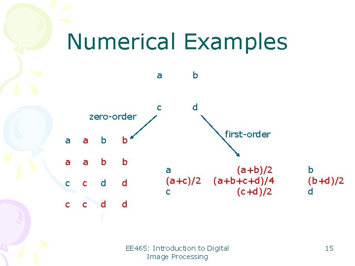
Numerical Examples zero-order a a b b c c d d a b c d first-order a (a+c)/2 c (a+b)/2 (a+b+c+d)/4 (c+d)/2 EE 465: Introduction to Digital Image Processing b (b+d)/2 d 15

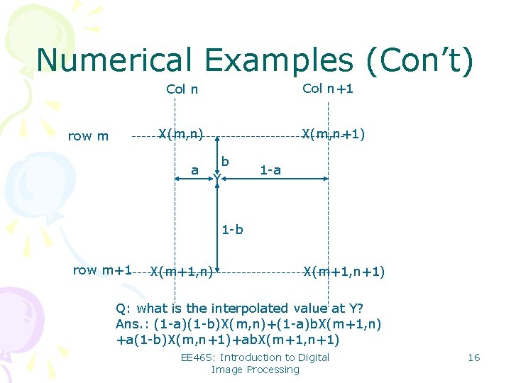
Numerical Examples (Con’t) Col n+1 Col n X(m, n) row m a X(m, n+1) b Y 1 -a 1 -b row m+1 X(m+1, n) X(m+1, n+1) Q: what is the interpolated value at Y? Ans. : (1 -a)(1 -b)X(m, n)+(1 -a)b. X(m+1, n) +a(1 -b)X(m, n+1)+ab. X(m+1, n+1) EE 465: Introduction to Digital Image Processing 16

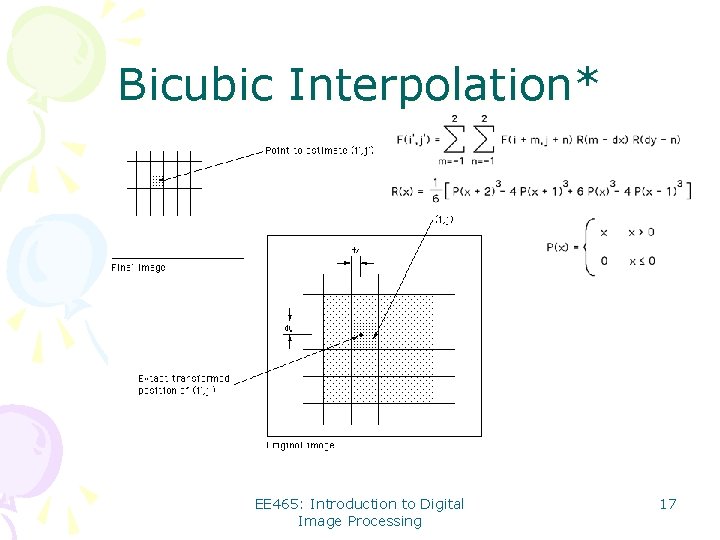
Bicubic Interpolation* EE 465: Introduction to Digital Image Processing 17

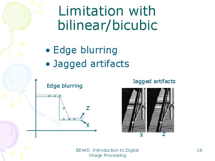
Limitation with bilinear/bicubic • Edge blurring • Jagged artifacts Edge blurring Z X X EE 465: Introduction to Digital Image Processing Z 18

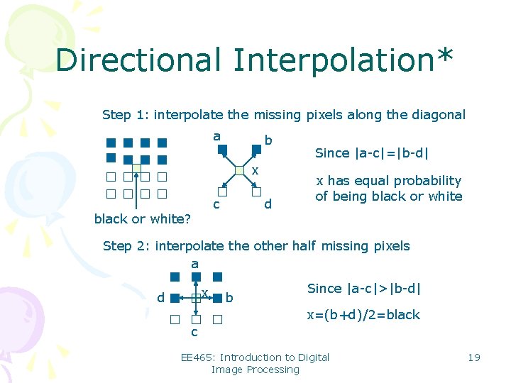
Directional Interpolation* Step 1: interpolate the missing pixels along the diagonal a b x c black or white? d Since |a-c|=|b-d| x has equal probability of being black or white Step 2: interpolate the other half missing pixels a x d b Since |a-c|>|b-d| x=(b+d)/2=black c EE 465: Introduction to Digital Image Processing 19

Image Interpolation • Introduction – What is image interpolation? – Why do we need it? • Interpolation Techniques – 1 D zero-order, first-order, third-order – 2 D zero-order, first-order, third-order – Directional interpolation* • Interpolation Applications – Digital zooming (resolution enhancement) – Image inpainting (error concealment) – Geometric transformations EE 465: Introduction to Digital Image Processing 20

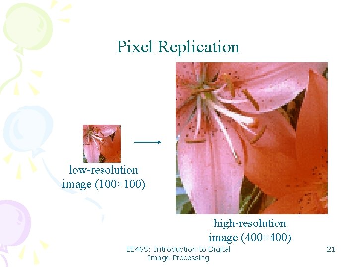
Pixel Replication low-resolution image (100× 100) high-resolution image (400× 400) EE 465: Introduction to Digital Image Processing 21

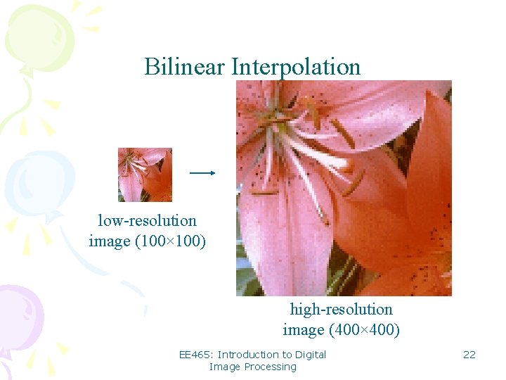
Bilinear Interpolation low-resolution image (100× 100) high-resolution image (400× 400) EE 465: Introduction to Digital Image Processing 22

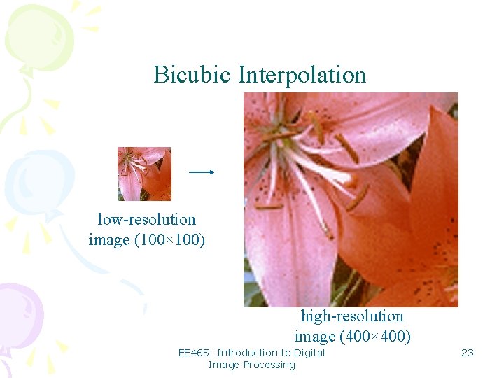
Bicubic Interpolation low-resolution image (100× 100) high-resolution image (400× 400) EE 465: Introduction to Digital Image Processing 23

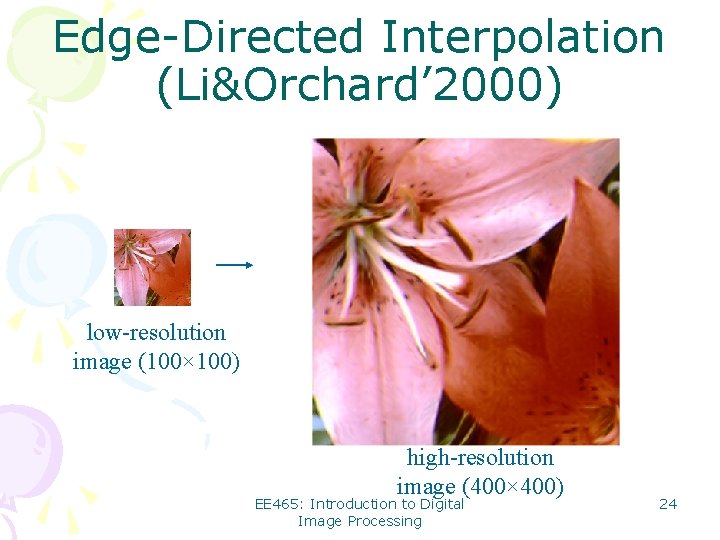
Edge-Directed Interpolation (Li&Orchard’ 2000) low-resolution image (100× 100) high-resolution image (400× 400) EE 465: Introduction to Digital Image Processing 24

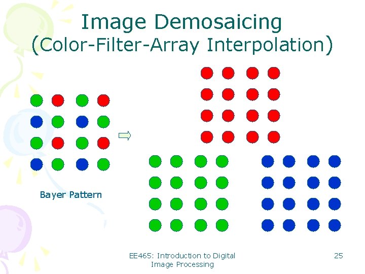
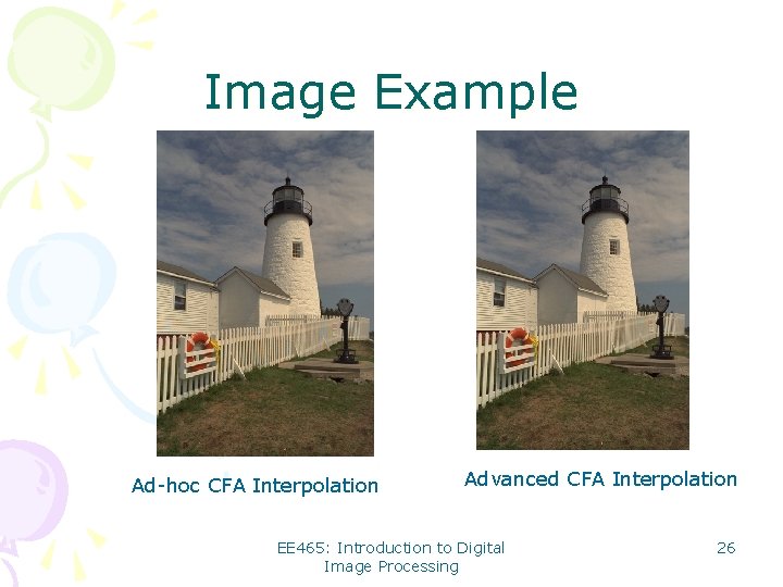
Image Demosaicing (Color-Filter-Array Interpolation) Bayer Pattern EE 465: Introduction to Digital Image Processing 25

Image Example Ad-hoc CFA Interpolation Advanced CFA Interpolation EE 465: Introduction to Digital Image Processing 26

Error Concealment damaged interpolated EE 465: Introduction to Digital Image Processing 27

Image Inpainting EE 465: Introduction to Digital Image Processing 28

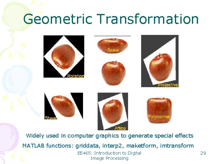
Geometric Transformation Widely used in computer graphics to generate special effects MATLAB functions: griddata, interp 2, maketform, imtransform EE 465: Introduction to Digital Image Processing 29

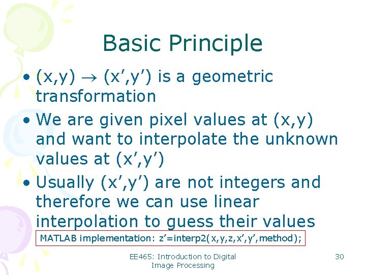
Basic Principle • (x, y) (x’, y’) is a geometric transformation • We are given pixel values at (x, y) and want to interpolate the unknown values at (x’, y’) • Usually (x’, y’) are not integers and therefore we can use linear interpolation to guess their values MATLAB implementation: z’=interp 2(x, y, z, x’, y’, method); EE 465: Introduction to Digital Image Processing 30

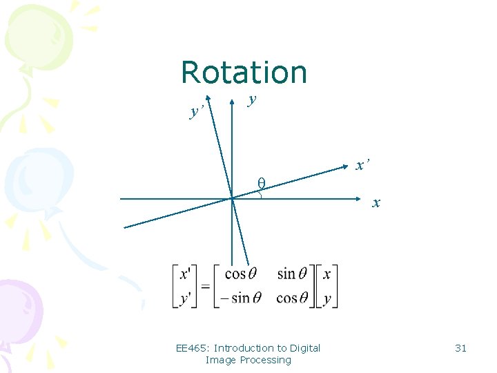
Rotation y’ y x’ θ x EE 465: Introduction to Digital Image Processing 31

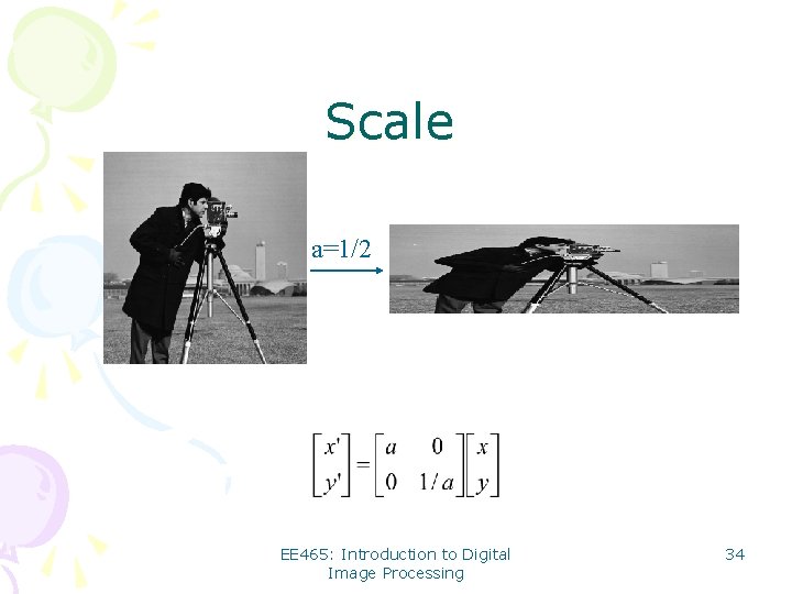
MATLAB Example z=imread('cameraman. tif'); % original coordinates [x, y]=meshgrid(1: 256, 1: 256); % new coordinates a=2; for i=1: 256; for j=1: 256; x 1(i, j)=a*x(i, j); y 1(i, j=y(i, j)/a; end % Do the interpolation z 1=interp 2(x, y, z, x 1, y 1, 'cubic'); EE 465: Introduction to Digital Image Processing 32

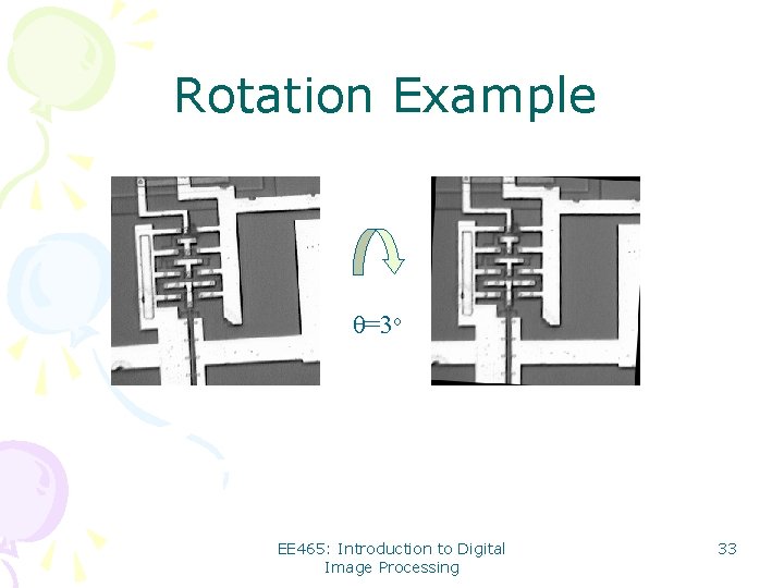
Rotation Example θ=3 o EE 465: Introduction to Digital Image Processing 33

Scale a=1/2 EE 465: Introduction to Digital Image Processing 34

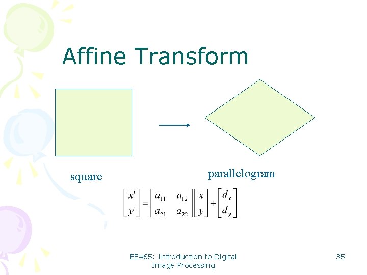
Affine Transform square parallelogram EE 465: Introduction to Digital Image Processing 35

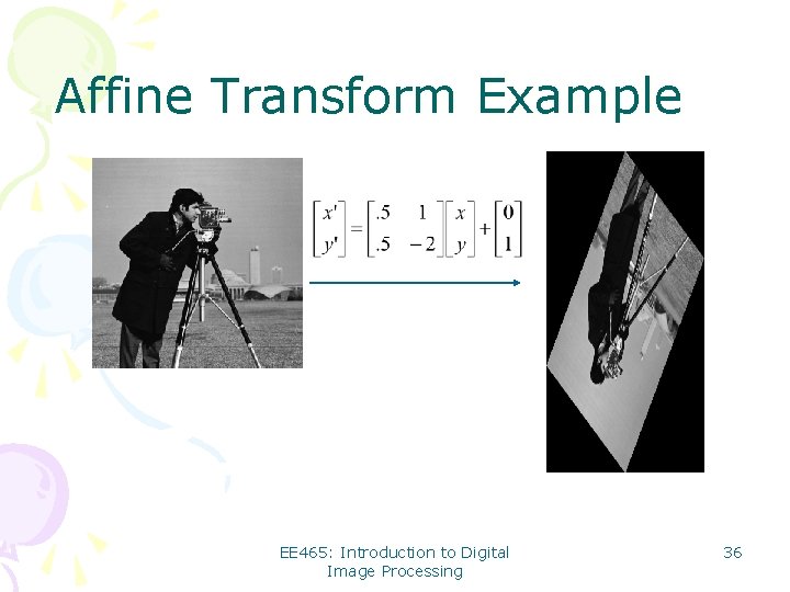
Affine Transform Example EE 465: Introduction to Digital Image Processing 36

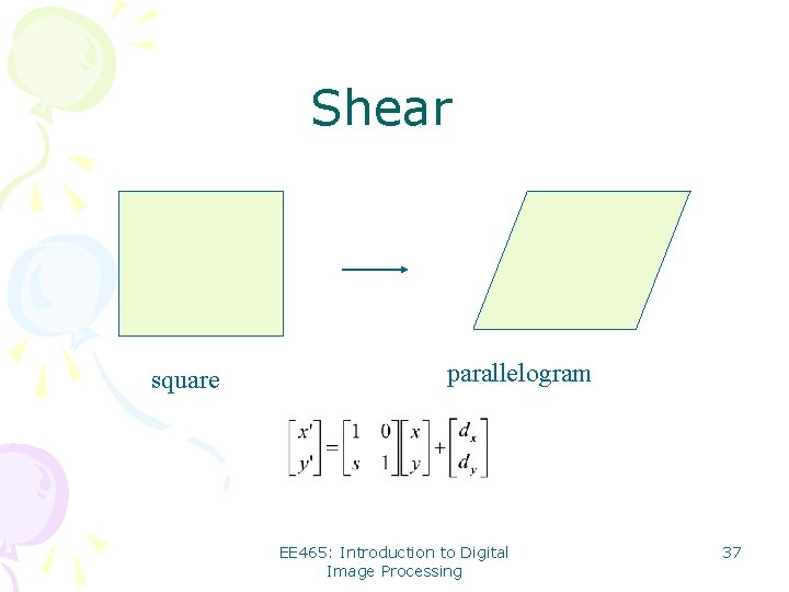
Shear square parallelogram EE 465: Introduction to Digital Image Processing 37

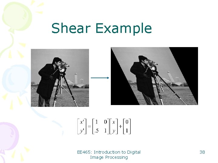
Shear Example EE 465: Introduction to Digital Image Processing 38

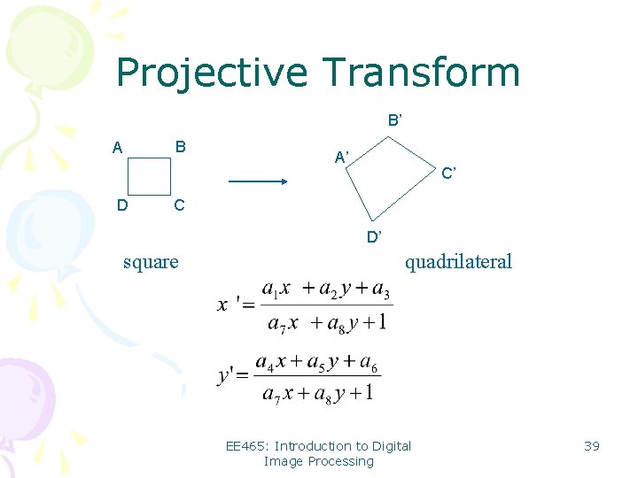
Projective Transform B’ B A D A’ C’ C D’ square quadrilateral EE 465: Introduction to Digital Image Processing 39

Projective Transform Example [ 0 0; 1 1; 0 1] [-4 2; -8 -3; -3 -5; 6 3] EE 465: Introduction to Digital Image Processing 40

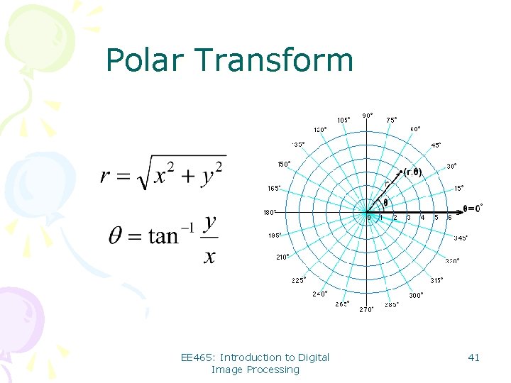
Polar Transform EE 465: Introduction to Digital Image Processing 41

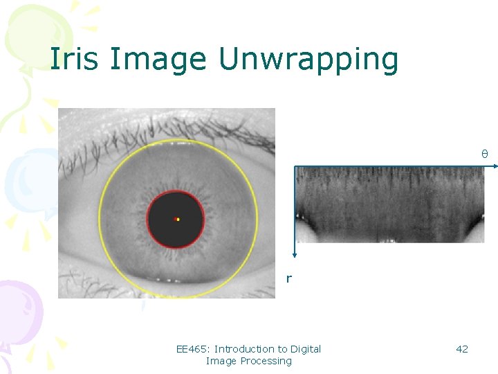
Iris Image Unwrapping r EE 465: Introduction to Digital Image Processing 42

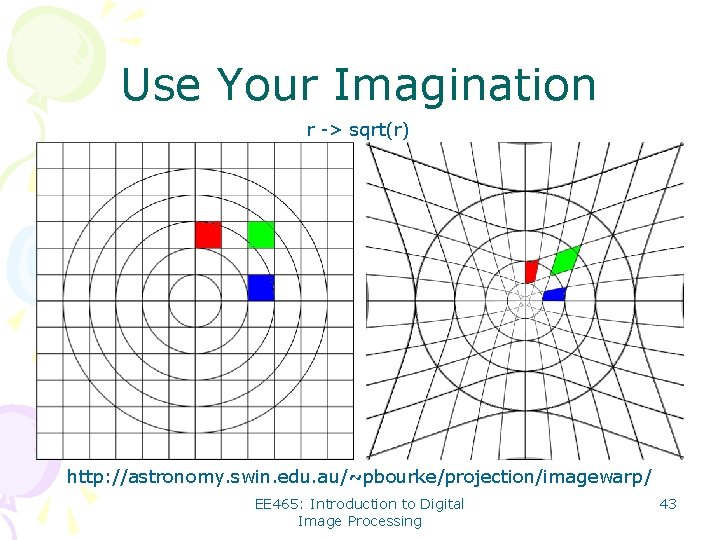
Use Your Imagination r -> sqrt(r) http: //astronomy. swin. edu. au/~pbourke/projection/imagewarp/ EE 465: Introduction to Digital Image Processing 43

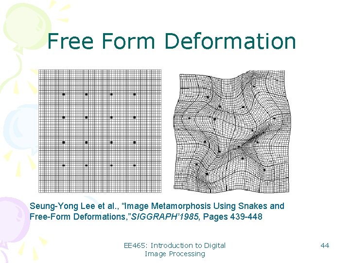
Free Form Deformation Seung-Yong Lee et al. , “Image Metamorphosis Using Snakes and Free-Form Deformations, ”SIGGRAPH’ 1985, Pages 439 -448 EE 465: Introduction to Digital Image Processing 44

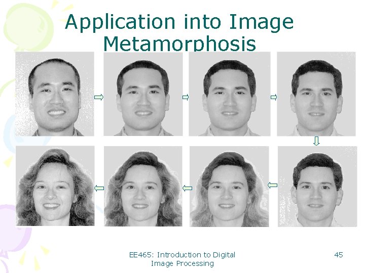
Application into Image Metamorphosis EE 465: Introduction to Digital Image Processing 45

Summary of Image Interpolation • A fundamental tool in digital processing of images: bridging the continuous world and the discrete world • Wide applications from consumer electronics to biomedical imaging • Remains a hot topic after the IT bubbles break EE 465: Introduction to Digital Image Processing 46