Numerical Analysis TOPIC Interpolation DEFINITION Interpolation is the

Numerical Analysis

TOPIC Interpolation

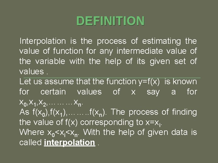
DEFINITION Interpolation is the process of estimating the value of function for any intermediate value of the variable with the help of its given set of values. Let us assume that the function y=f(x) is known for certain values of x say a for x 0, x 1, x 2, ………xn. As f(x 0), f(x 1), ……. . f(xn). The process of finding the value of f(x) corresponding to x=xi. Where x 0<xi<xn. With the help of given data is called interpolation.

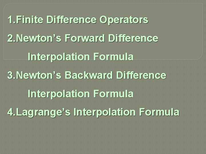
TYPES OF INTERPOLATION

1. Finite Difference Operators 2. Newton’s Forward Difference Interpolation Formula 3. Newton’s Backward Difference Interpolation Formula 4. Lagrange’s Interpolation Formula

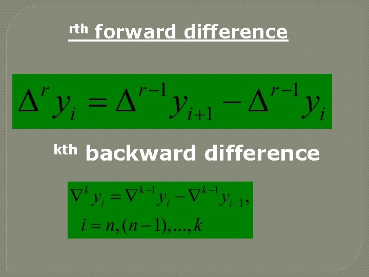
rth kth forward difference backward difference

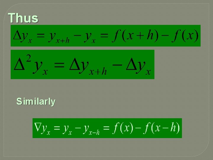
Thus Similarly

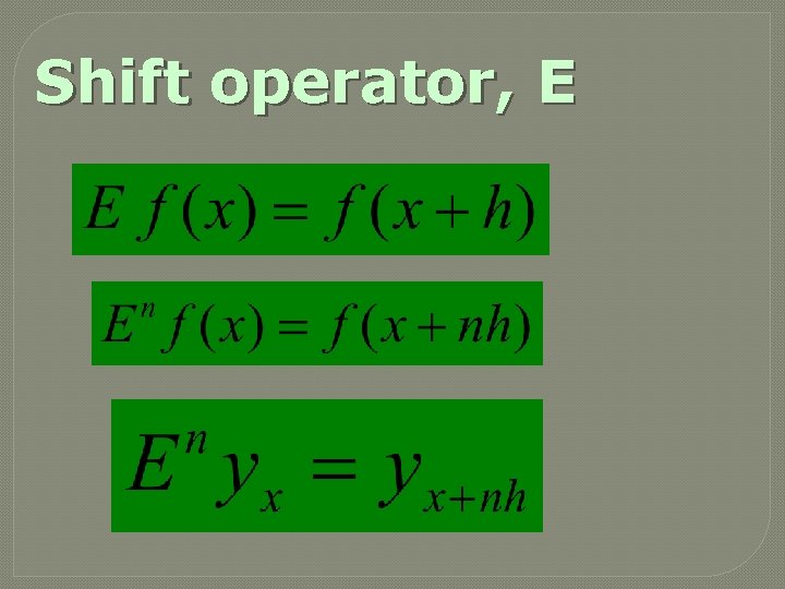
Shift operator, E

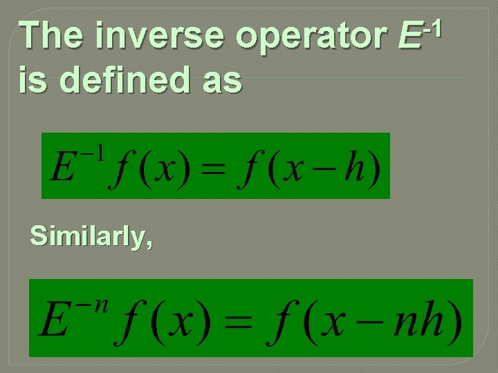
The inverse operator is defined as Similarly, -1 E

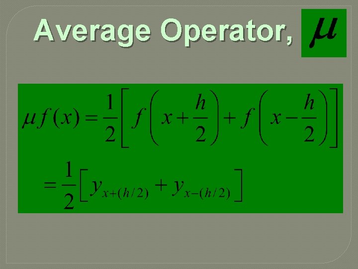
Average Operator,

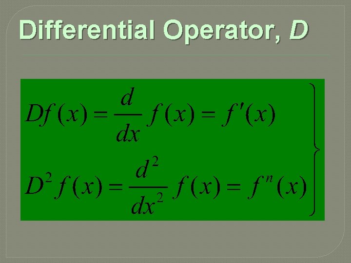
Differential Operator, D

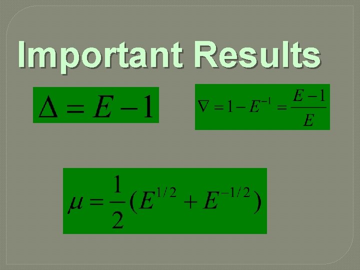
Important Results

Newton’s Forward Difference Interpolation Formula

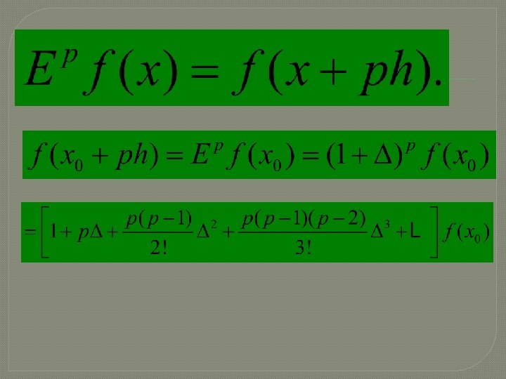
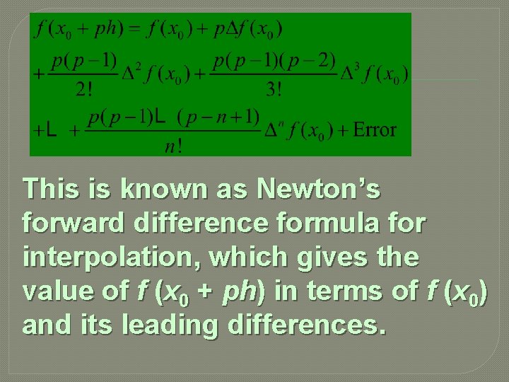
Let y = f (x) be a function which takes values f (x 0), f (x 0+ h), f (x 0+2 h), …, corresponding to various equispaced values of x with spacing h, say x 0, x 0 + h, x 0 + 2 h, …. Suppose, we wish to evaluate the function f (x) for a value x 0 + ph, where p is any real number, then for any real number p, we have the operator E such that

This is known as Newton’s forward difference formula for interpolation, which gives the value of f (x 0 + ph) in terms of f (x 0) and its leading differences.

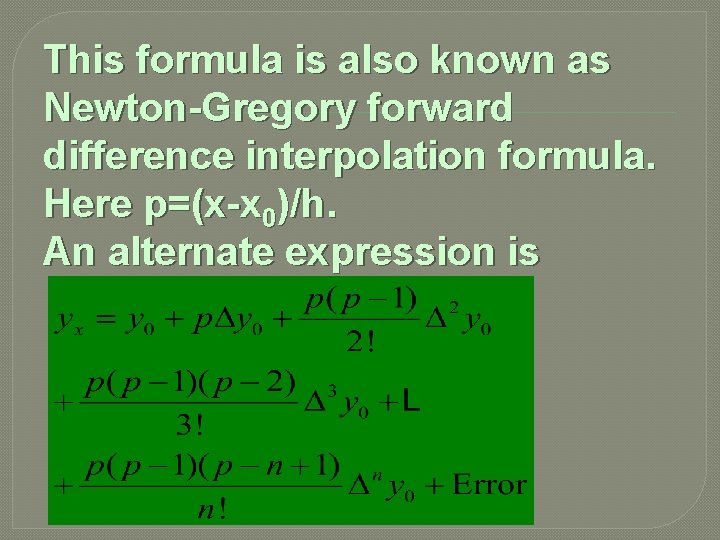
This formula is also known as Newton-Gregory forward difference interpolation formula. Here p=(x-x 0)/h. An alternate expression is

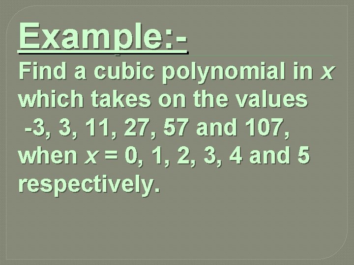
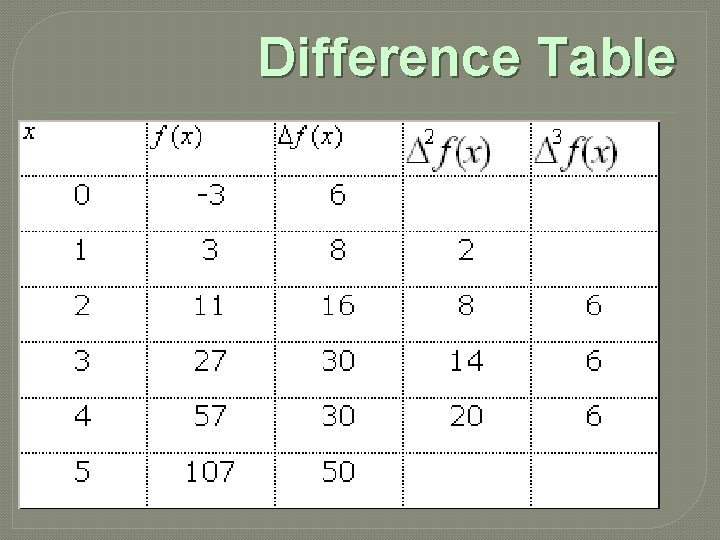
Example: Find a cubic polynomial in x which takes on the values -3, 3, 11, 27, 57 and 107, when x = 0, 1, 2, 3, 4 and 5 respectively.

Solution: Here, the observations are given at equal intervals of unit width. To determine the required polynomial, we first construct the difference table

Difference Table

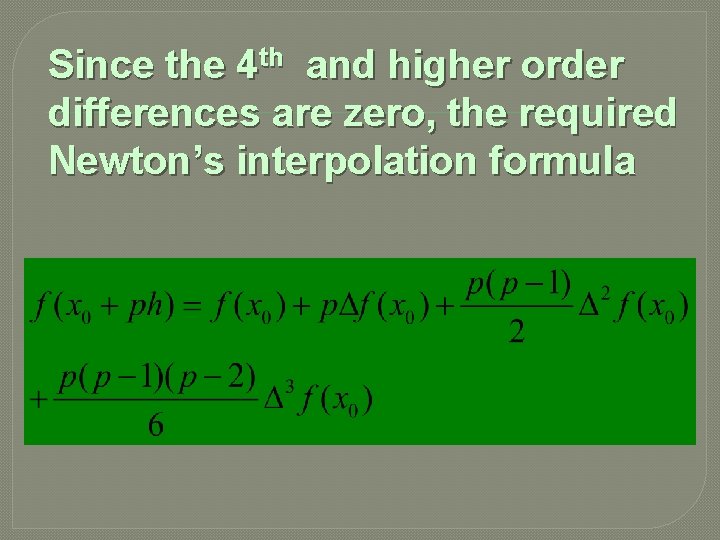
Since the 4 th and higher order differences are zero, the required Newton’s interpolation formula

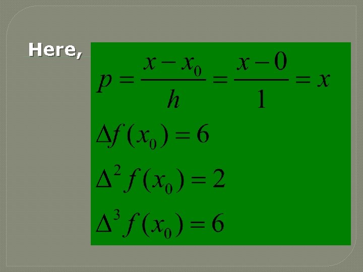
Here,

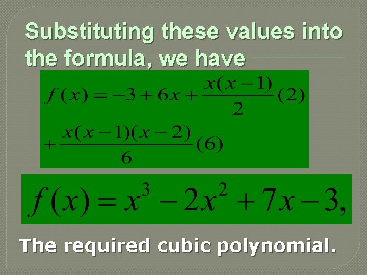
Substituting these values into the formula, we have The required cubic polynomial.

NEWTON’S BACKWARD DIFFERENCE INTERPOLATION FORMULA

For interpolating the value of the function y = f (x) near the end of table of values, and to extrapolate value of the function a short distance forward from yn, Newton’s backward interpolation formula is used

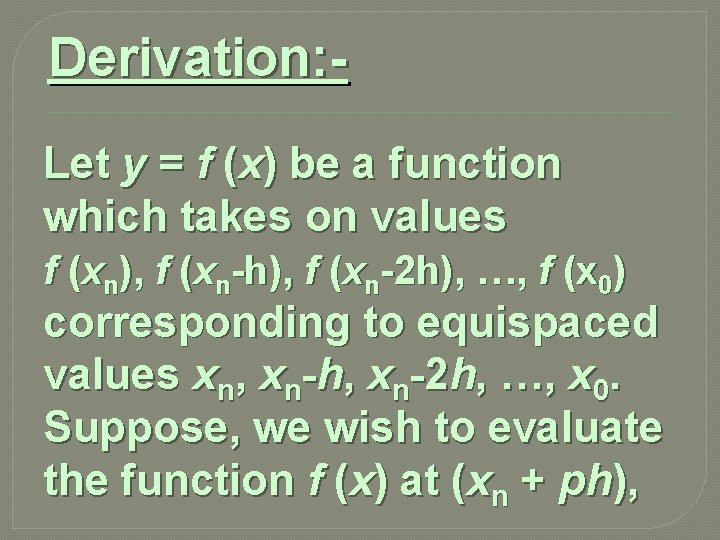
Derivation: Let y = f (x) be a function which takes on values f (xn), f (xn-h), f (xn-2 h), …, f (x 0) corresponding to equispaced values xn, xn-h, xn-2 h, …, x 0. Suppose, we wish to evaluate the function f (x) at (xn + ph),

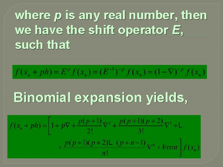
where p is any real number, then we have the shift operator E, such that Binomial expansion yields,

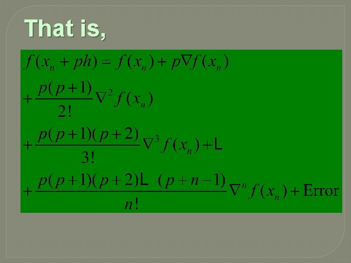
That is,

This formula is known as Newton’s backward interpolation formula. This formula is also known as Newton’s-Gregory backward difference interpolation formula.

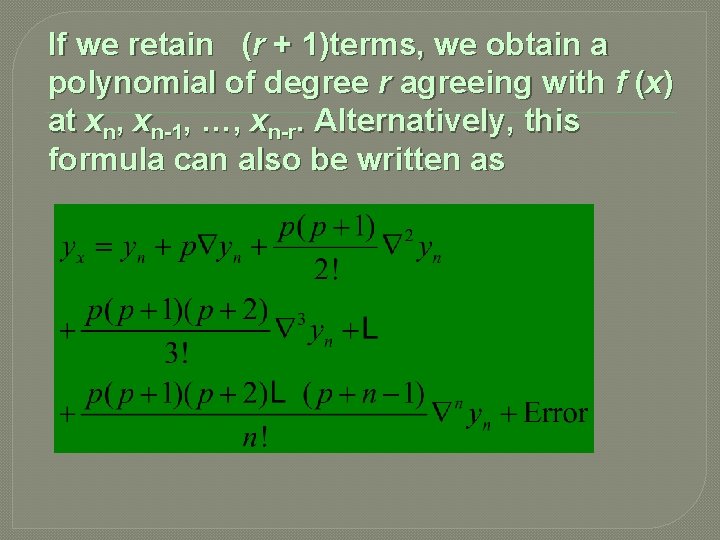
If we retain (r + 1)terms, we obtain a polynomial of degree r agreeing with f (x) at xn, xn-1, …, xn-r. Alternatively, this formula can also be written as

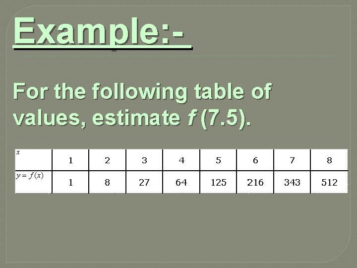
Example: For the following table of values, estimate f (7. 5).

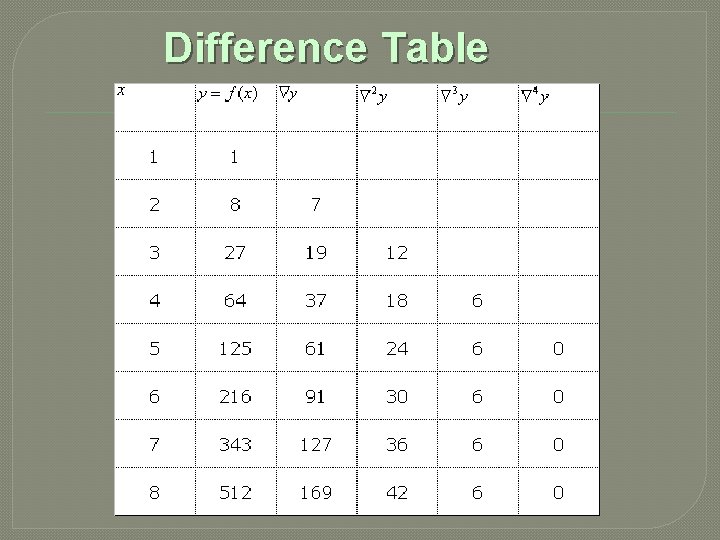
Solution: The value to be interpolated is at the end of the table. Hence, it is appropriate to use Newton’s backward interpolation formula. Let us first construct the backward difference table for the given data

Difference Table

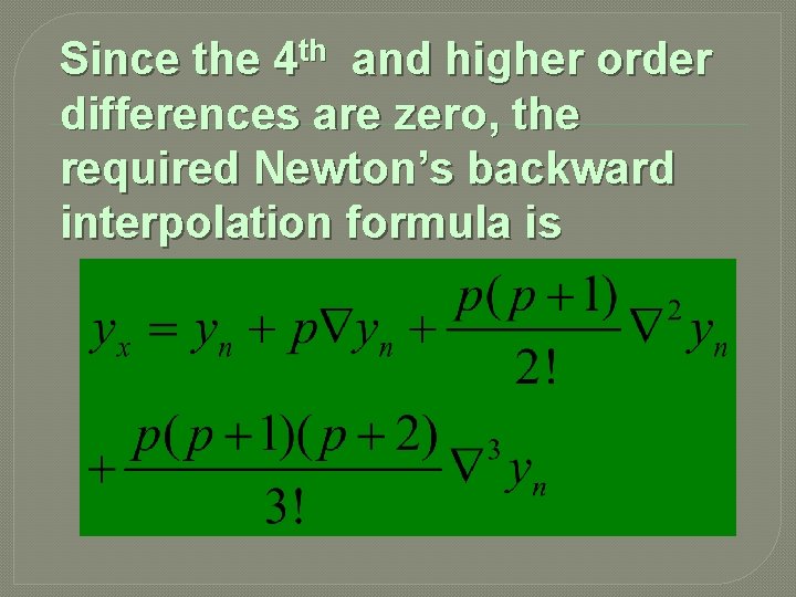
Since the 4 th and higher order differences are zero, the required Newton’s backward interpolation formula is

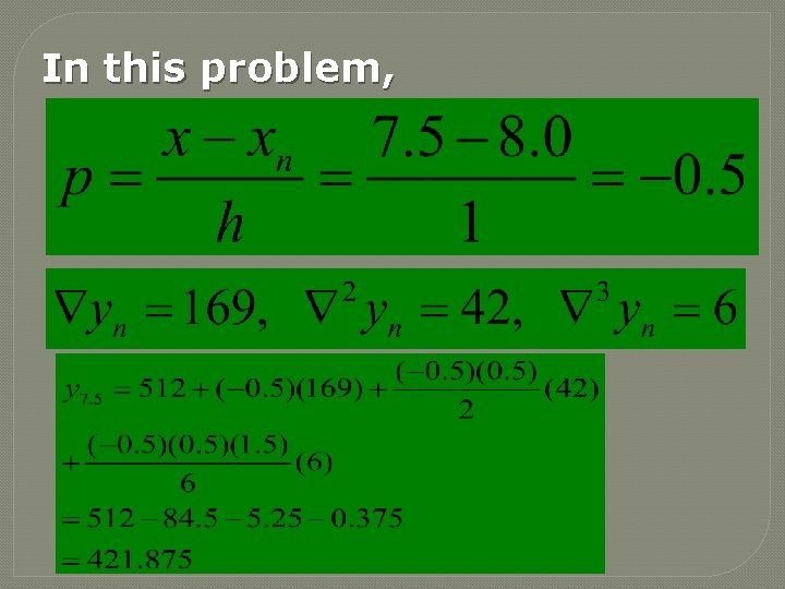
In this problem,

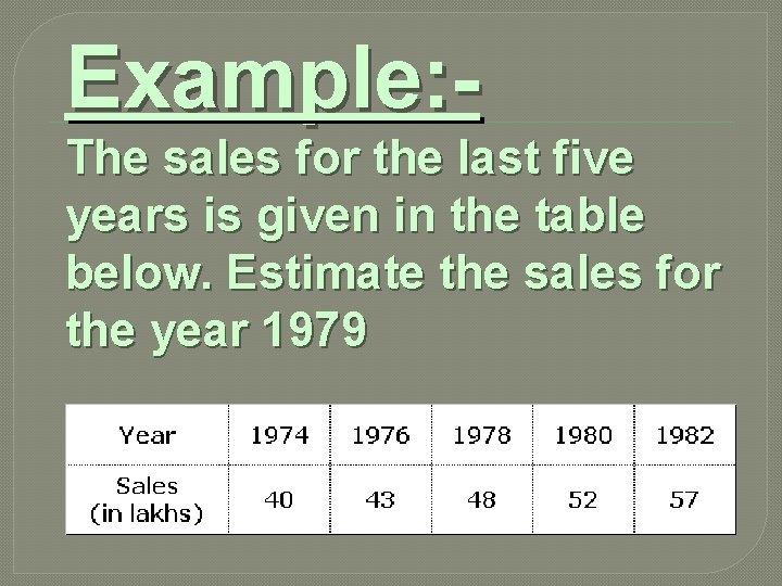
Example: The sales for the last five years is given in the table below. Estimate the sales for the year 1979

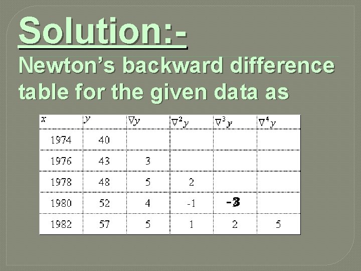
Solution: Newton’s backward difference table for the given data as -3

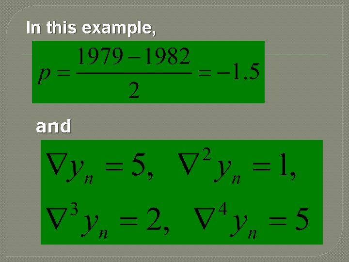
In this example, and

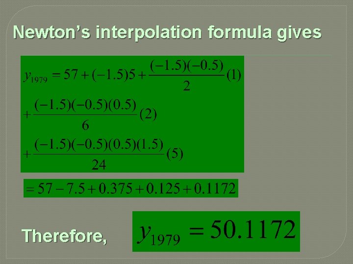
Newton’s interpolation formula gives Therefore,

LAGRANGE’S INTERPOLATION FORMULA

Newton’s interpolation formulae developed earlier can be used only when the values of the independent variable x are equally spaced. Also the differences of y must ultimately become small.

If the values of the independent variable are not given at equidistant intervals, then we have the basic formula associated with the name of Lagrange which will be derived now.

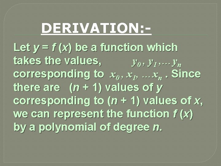
DERIVATION: Let y = f (x) be a function which takes the values, y 0 , y 1 , …yn corresponding to x 0 , x 1, …xn. Since there are (n + 1) values of y corresponding to (n + 1) values of x, we can represent the function f (x) by a polynomial of degree n.

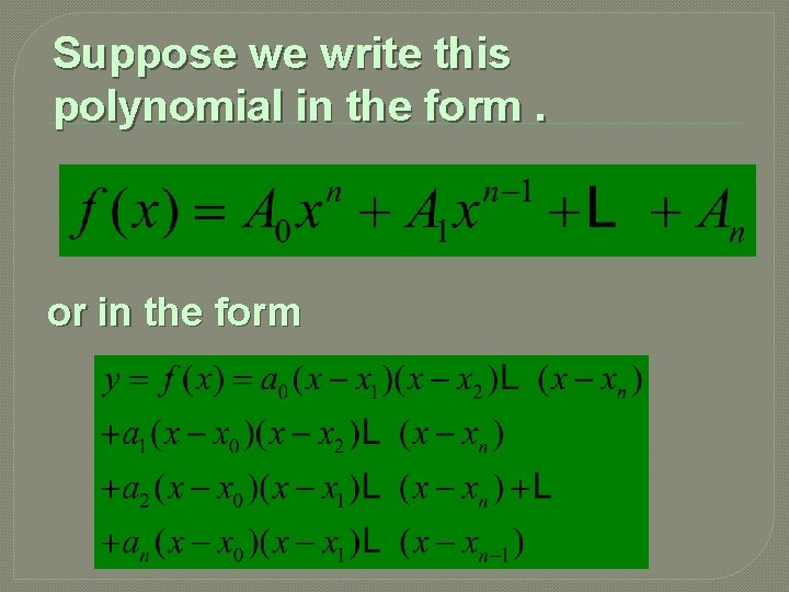
Suppose we write this polynomial in the form. or in the form

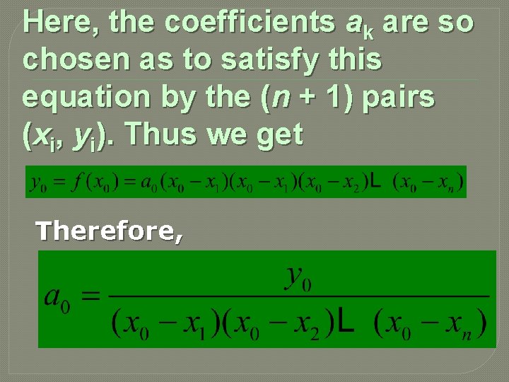
Here, the coefficients ak are so chosen as to satisfy this equation by the (n + 1) pairs (xi, yi). Thus we get Therefore,

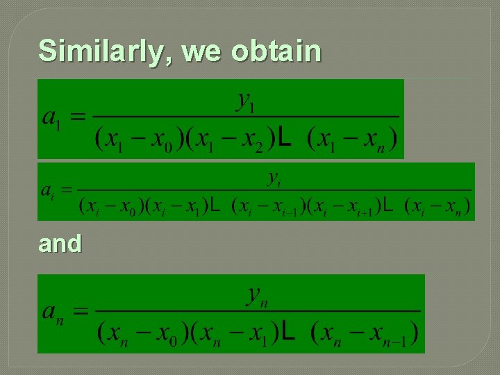
Similarly, we obtain and

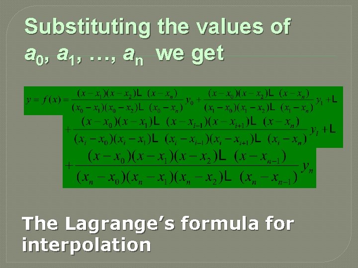
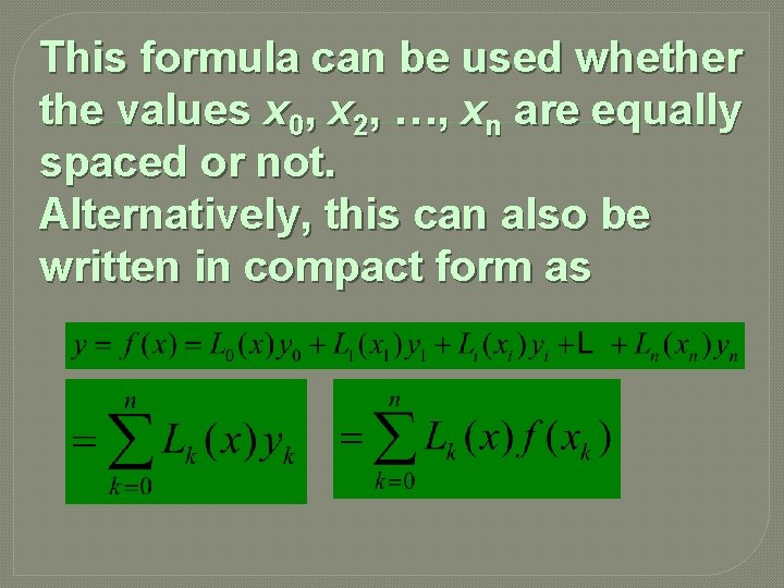
Substituting the values of a 0, a 1, …, an we get The Lagrange’s formula for interpolation

This formula can be used whether the values x 0, x 2, …, xn are equally spaced or not. Alternatively, this can also be written in compact form as

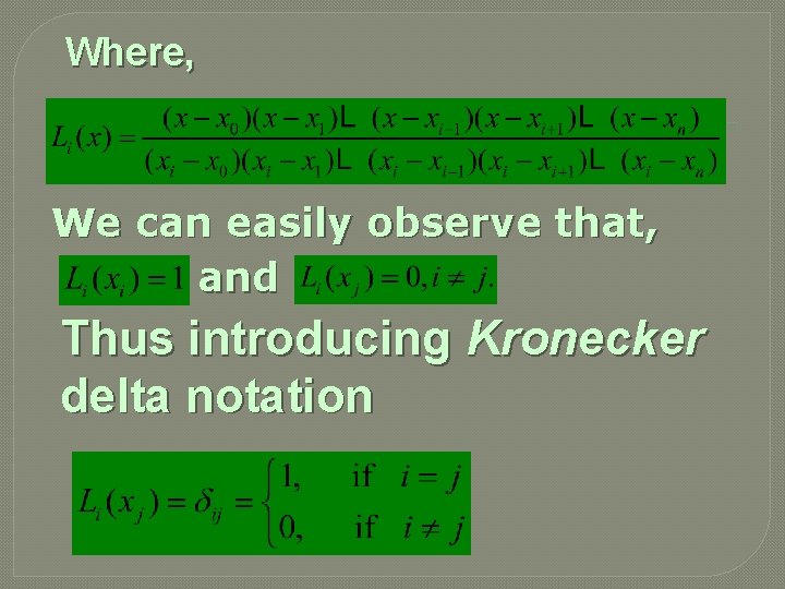
Where, We can easily observe that, and Thus introducing Kronecker delta notation

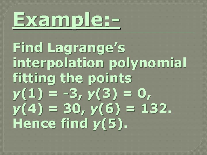
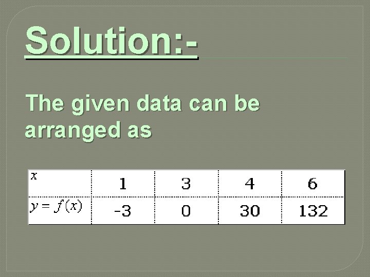
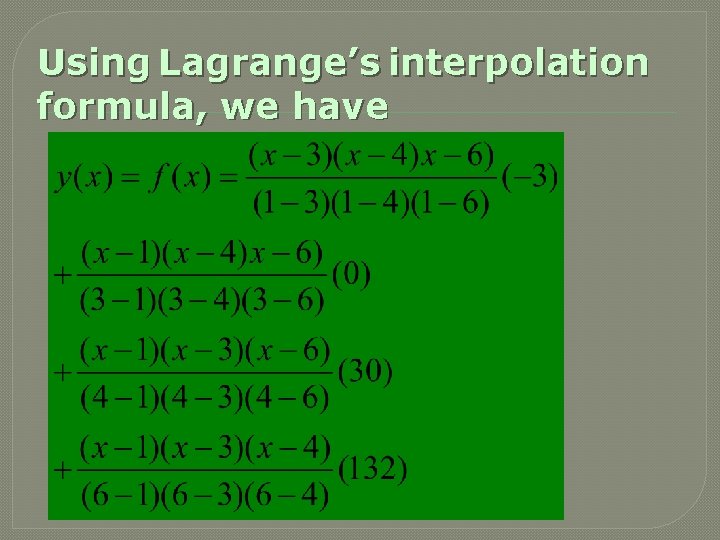
Example: Find Lagrange’s interpolation polynomial fitting the points y(1) = -3, y(3) = 0, y(4) = 30, y(6) = 132. Hence find y(5).

Solution: The given data can be arranged as

Using Lagrange’s interpolation formula, we have

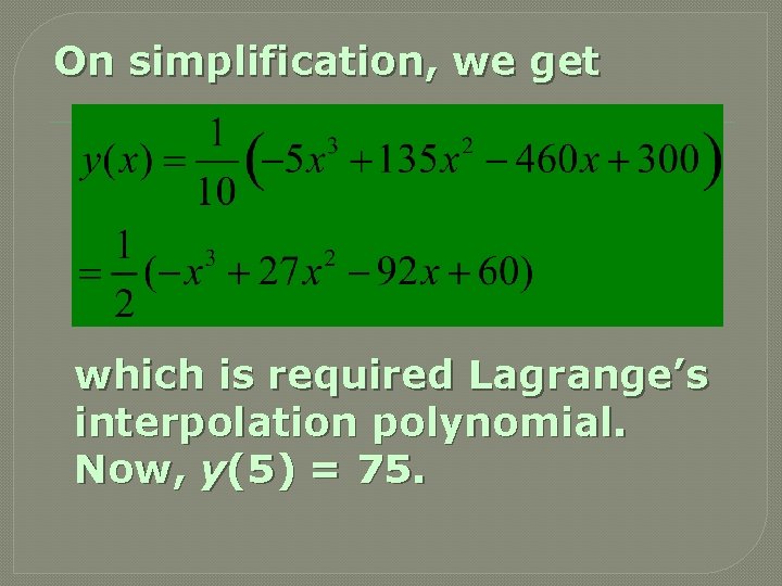
On simplification, we get which is required Lagrange’s interpolation polynomial. Now, y(5) = 75.

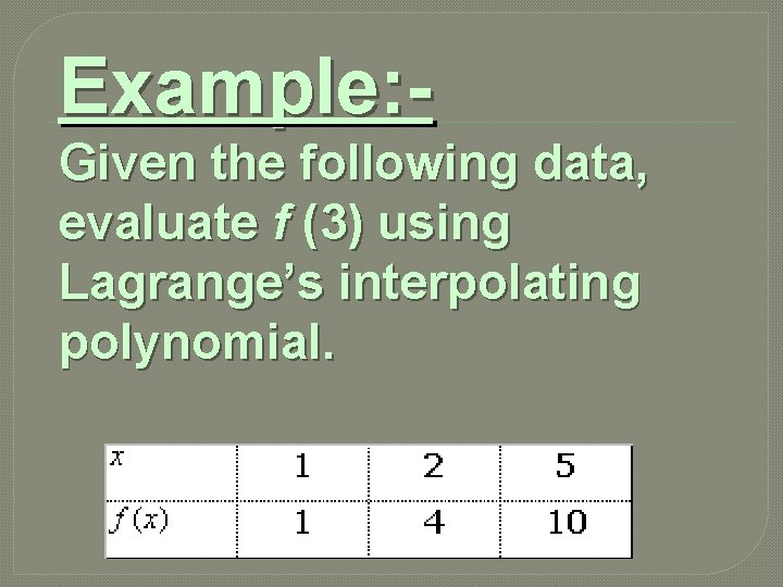
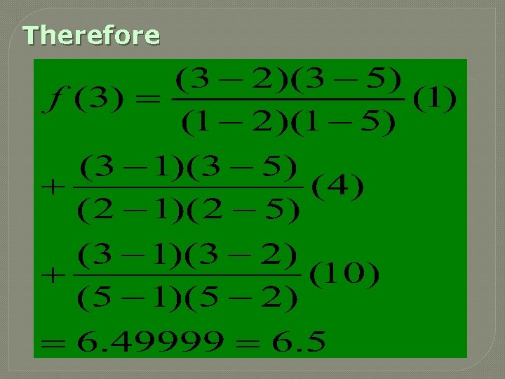
Example: Given the following data, evaluate f (3) using Lagrange’s interpolating polynomial.

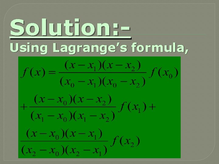
Solution: - Using Lagrange’s formula,

Therefore

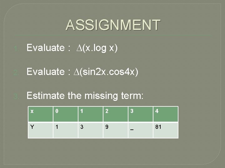
ASSIGNMENT 1. Evaluate : (x. log x) 2. Evaluate : (sin 2 x. cos 4 x) 3. Estimate the missing term: x 0 1 2 3 4 Y 1 3 9 _ 81

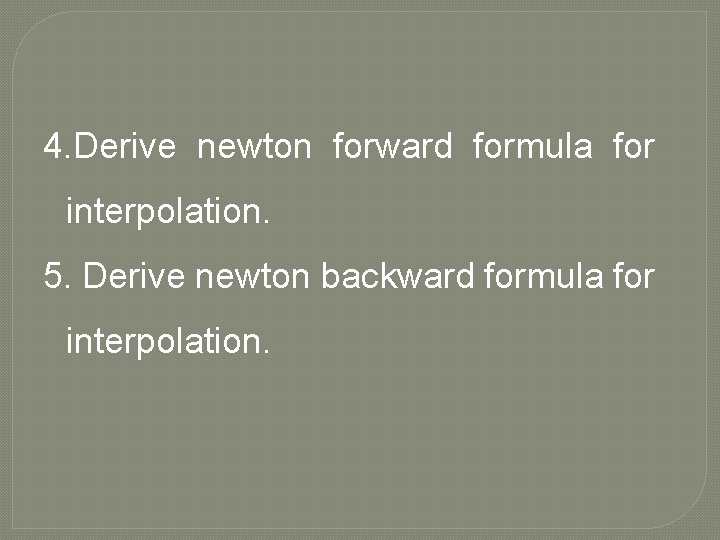
4. Derive newton forward formula for interpolation. 5. Derive newton backward formula for interpolation.

TEST NOTE: DO ANY TWO

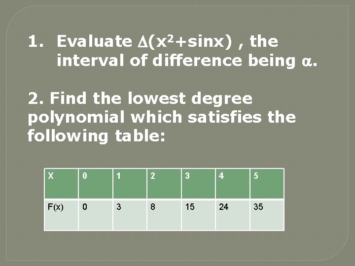
1. Evaluate (x 2+sinx) , the interval of difference being . 2. Find the lowest degree polynomial which satisfies the following table: X 0 1 2 3 4 5 F(x) 0 3 8 15 24 35

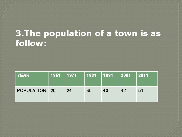
3. The population of a town is as follow: YEAR 1961 POPULATION 20 1971 1981 1991 2001 2011 24 35 40 42 51