Interpolation A standard idea in interpolation now is

Interpolation A standard idea in interpolation now is to find a polynomial pn(x) of degree n (or less) that assumes the given values; thus (1) We call this pn(x) an interpolation polynomial and x 0, ‥‥, xn the nodes. And if ƒ(x) is a mathematical function, we call pn(x) a polynomial approximation of ƒ. We use pn(x) to get (approximate) values of ƒ for x’s between x 0 and xn (“interpolation”) or sometimes outside this interval (“extrapolation”). 歐亞書局 P 797 continued

Lagrange Interpolation Linear interpolation is interpolation by the straight line through (x 0, ƒ 0), (x 1, ƒ 1); see Fig. 428. Thus the linear Lagrange polynomial p 1 is a sum p 1 = L 0ƒ 0 + L 1ƒ 1 with L 0 the linear polynomial that is 1 at x 0 and 0 at x 1; similarly, L 1 is 0 at x 0 and 1 at x 1. Obviously, This gives the linear Lagrange polynomial (2) 歐亞書局 P 798 continued

Fig. 428. 歐亞書局 P 798 Linear interpolation

¬ Thus |εn(x)| is 0 at the nodes and small near them, because of continuity. The product (x – x 0) ‥‥ (x – xn) is large for x away from the nodes. This makes extrapolation risky. And interpolation at an x will be best if we choose nodes on both sides of that x. Also, we get error bounds by taking the smallest and the largest value of ƒ(n+1)(t) in (5) on the interval x 0 ≤ t ≤ xn (or on the interval also containing x if we extrapolate). ¬ Most importantly, since pn is unique, as we have shown, we have 歐亞書局 P 800

E X A M P L E 1 Linear Lagrange Interpolation Compute a 4 D-value of ln 9. 2 from ln 9. 0 = 2. 1972, ln 9. 5 = 2. 2513 by linear Lagrange interpolation and determine the error, using ln 9. 2 = 2. 2192 (4 D). Solution. x 0 = 9. 0, x 1 = 9. 5, ƒ 0 = ln 9. 0, ƒ 1 = ln 9. 5. In (2) we need and obtain the answer 歐亞書局 P 798 continued

The error is ε = a – a = 2. 2192 – 2. 2188 = 0. 0004. Hence linear interpolation is not sufficient here to get 4 Daccuracy; it would suffice for 3 D-accuracy. 歐亞書局 P 798 continued

Fig. 429. 歐亞書局 P 799 L 0 and L 1 in Example 1

Quadratic interpolation The interpolation of given (x 0, ƒ 0), (x 1, ƒ 1), (x 2, ƒ 2) by a seconddegree polynomial p 2(x), which by Lagrange’s idea is (3 a) with L 0(x 0) = 1, L 1(x 1) = 1, L 2(x 2) = 1, and L 0(x 1) = L 0(x 2) = 0, etc. We claim that (3 b) 歐亞書局 P 799 continued

E X A M P L E 2 Quadratic Lagrange Interpolation Compute ln 9. 2 by (3) from the data in Example 1 and the additional third value ln 11. 0 = 2. 3979. Solution. In (3), so that (3 a) gives, exact to 4 D, 歐亞書局 P 799 continued

Fig. 430. 歐亞書局 P 799 L 0, L 1, L 2 in Example 2

General Lagrange Interpolation Polynomial For general n we obtain (4 a) where Lk(xk) = 1 and Lk is 0 at the other nodes, and the Lk are independent of the function ƒ to be interpolated. We get (4 a) if we take (4 b) We can easily see that pn(xk) = ƒk. 歐亞書局 P 800 continued

Error Estimate If ƒ is itself a polynomial of degree n (or less), it must coincide with pn because the n + 1 data (x 0, ƒ 0), ‥‥, (xn, ƒn) determine a polynomial uniquely, so the error is zero. Now the special ƒ has its (n + 1)st derivative identically zero. This makes it plausible that for a general ƒ its (n + 1)st derivative ƒ(n+1) should measure the error If ƒ(n+1) exists and is continuous, then with a suitable t between x 0 and xn (5) 歐亞書局 P 800 continued

THEOREM 1 Error of Interpolation Formula (5) gives the error for any polynomial interpolation method if ƒ(x) has a continuous (n + 1)st derivative. 歐亞書局 P 800

E X A M P L E 3 Error Estimate (5) of Linear Interpolation. Damage by Roundoff. Error Principle ¬ Estimate the error in Example 1 first by (5) directly and then by the Error Principle (Sec. 19. 1). ¬ Solution. (A) Estimation by (5). We have n = 1, ƒ(t) = ln t, ƒ'(t) = 1/t, ƒ"(t) = – 1/t 2. Hence t = 9. 0 gives the maximum 0. 03/92 = 0. 00037 and t = 9. 5 gives the minimum 0. 03/9. 52 = 0. 00033, so that we get 0. 00033 ≤ ε 1(9. 2) ≤ 0. 00037, or better, 0. 00038 because 0. 3/81 = 0. 003 703 ‥‥. 歐亞書局 P 801 continued

¬ But the error 0. 0004 in Example 1 disagrees, and we can learn something! Repetition of the computation there with 5 D instead of 4 D gives with an actual error ε = 2. 21920 – 2. 21885 = 0. 00035, which lies nicely near the middle between our two error bounds. ¬ This shows that the discrepancy (0. 0004 vs. 0. 00035) was caused by rounding, which is not taken into account in (5). 歐亞書局 P 801 continued

¬ (B) Estimation by the Error Principle. We calculate p 1(9. 2) = 2. 21885 as before and then p 2(9. 2) as in Example 2 but with 5 D, obtaining ¬ The difference p 2(9. 2) – p 1(9. 2) = 0. 00031 is the approximate error of p 1(9. 2) that we wanted to obtain; this is an approximation of the actual error 0. 00035 given above. 歐亞書局 P 801

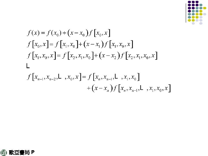
Newton’s Divided Difference Interpolation The kth divided difference, recursively denoted and defined as follows: and in general (8) 歐亞書局 P 802

With p 0(x) = ƒ 0 by repeated application with k = 1, ‥‥, n this finally gives Newton’s divided difference interpolation formula (10) 歐亞書局 P 802

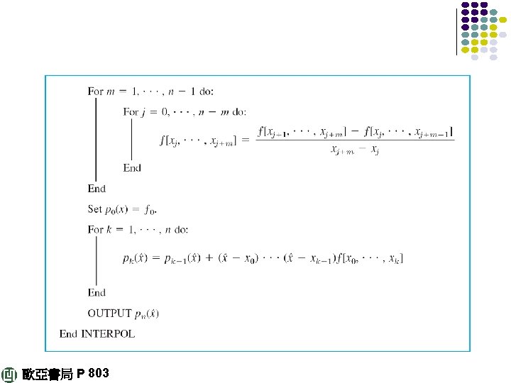
Table 19. 2 Newton’s Divided Difference Interpolation 歐亞書局 P 803 continued

E X A M P L E 4 Newton’s Divided Difference Interpolation Formula Compute ƒ(9. 2) from the values shown in the first two columns of the following table. 歐亞書局 P 803 continued

Solution We compute the divided differences as shown. Sample computation: The values we need in (10) are circled. We have The value exact to 6 D is ƒ(9. 2) = ln 9. 2 = 2. 219 203. Note that we can nicely see how the accuracy increases from term to term: 歐亞書局 P 804 continued

Equal Spacing: Newton’s Forward Difference Formula Newton’s formula (10) is valid for arbitrarily spaced nodes as they may occur in practice in experiments or observations. However, in many applications the xj’s are regularly spaced— for instance, in measurements taken at regular intervals of time. Then, denoting the distance by h, we can write (11) We can show (8) and (10) now simplify considerably! 歐亞書局 P 804 continued

Let us define the first forward difference of ƒ at xj by and the second forward difference of ƒ at xj by and, continuing in this way, the kth forward difference of ƒ at xj by (12) 歐亞書局 P 804

Formula (10) becomes Newton’s (or Gregory–Newton’s) forward difference interpolation formula (14) where the binomial coefficients in the first line are defined by (15) and s! = 1 • 2 ‥‥ s. 歐亞書局 P 805 continued

Error From (5) we get, with x – x 0 = rh, x – x 1 = (r – 1)h, etc. , (16) with t as characterized in (5). 歐亞書局 P 805

E X A M P L E 5 Newton’s Forward Difference Formula. Error Estimation Compute cosh 0. 56 from (14) and the four values in the following table and estimate the error. 歐亞書局 P 806 continued

Solution We compute the forward differences as shown in the table. The values we need are circled. In (14) we have r = (0. 56 – 0. 50)/0. 1 = 0. 6, so that (14) gives 歐亞書局 P 806 continued

Error estimate. From (16), since the fourth derivative is cosh(4) t = cosh t, where A = – 0. 000 003 36 and 0. 5 ≤ t ≤ 0. 8. We do not know t, but we get an inequality by taking the largest and smallest cosh t in that interval: 歐亞書局 P 806 continued

Since this gives Numeric values are The exact 6 D-value is cosh 0. 56 = 1. 160 941. It lies within these bounds. Such bounds are not always so tight. Also, we did not consider roundoff errors, which will depend on the number of operations. 歐亞書局 P 806

Equal Spacing: Newton’s Backward Difference Formula A formula similar to (14) but involving backward differences is Newton’s (or Gregory–Newton’s) backward difference interpolation formula (18) 歐亞書局 P 807

E X A M P L E 6 Newton’s Forward and Backward Interpolations Compute a 7 D-value of the Bessel function J 0(x) for x = 1. 72 from the four values in the following table, using (a) Newton’s forward formula (14), (b) Newton’s backward formula (18). 歐亞書局 P 807 continued

Solution. The computation of the differences is the same in both cases. Only their notation differs. (a) Forward. In (14) we have r = (1. 72 – 1. 70)/0. 1 = 0. 2, and j goes from 0 to 3 (see first column). In each column we need the first given number, and (14) thus gives which is exact to 6 D, the exact 7 D-value being 0. 386 4185. 歐亞書局 P 807 continued

(b) Backward. For (18) we use j shown in the second column, and in each column the last number. Since r = (1. 72 – 2. 00)/ 0. 1 = – 2. 8, we thus get from (18) 歐亞書局 P 808

Central Difference Notation This is a third notation for differences. The first central difference of ƒ(x) at xj is defined by and the kth central difference of ƒ(x) at xj by (19) 歐亞書局 P 808