Lecture 9 Interpolation and Splines Lingo Interpolation filling

Lecture 9 Interpolation and Splines

Lingo Interpolation – filling in gaps in data Find a function f(x) that 1) goes through all your data points 2) does something sensible in between

Lingo Splines – a broad class of ways of performing interpolation (we’ll get to the details, eventually)

Find a function f(x) that 1) goes through all your data points (observations) 2) does something sensible in between (prior information) Why not just use least-squares?

Remember this? mest = m. A + M [ dobs – Gm. A] where M = [GTCd-1 G + Cm-1]-1 GT Cd-1

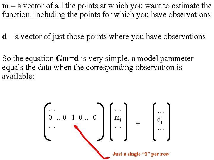
m – a vector of all the points at which you want to estimate the function, including the points for which you have observations d – a vector of just those points where you have observations So the equation Gm=d is very simple, a model parameter equals the data when the corresponding observation is available: … 0… 0 1 0… 0 … … mi … = … dj … Just a single “ 1” per row

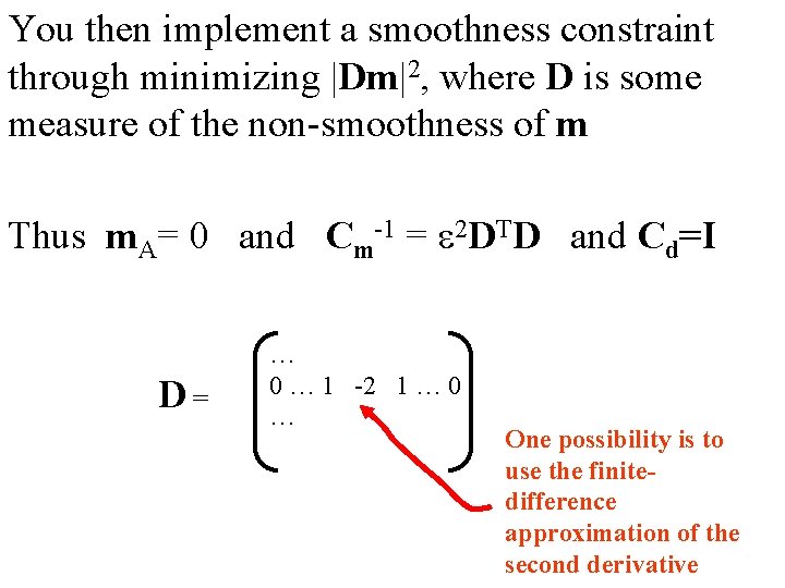
You then implement a smoothness constraint through minimizing |Dm|2, where D is some measure of the non-smoothness of m Thus m. A= 0 and Cm-1 = e 2 DTD and Cd=I D= … 0 … 1 -2 1 … 0 … One possibility is to use the finitedifference approximation of the second derivative

First derivative [dm/dx]i (1/Dx) mi – mi-1 Second derivative [d 2 m/dx 2]i [dm/dx]i+1 - [dm/dx]i = mi+1 – mi + mi-1 = mi+1 – 2 mi + mi-1

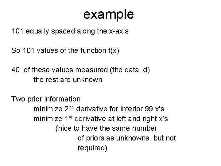
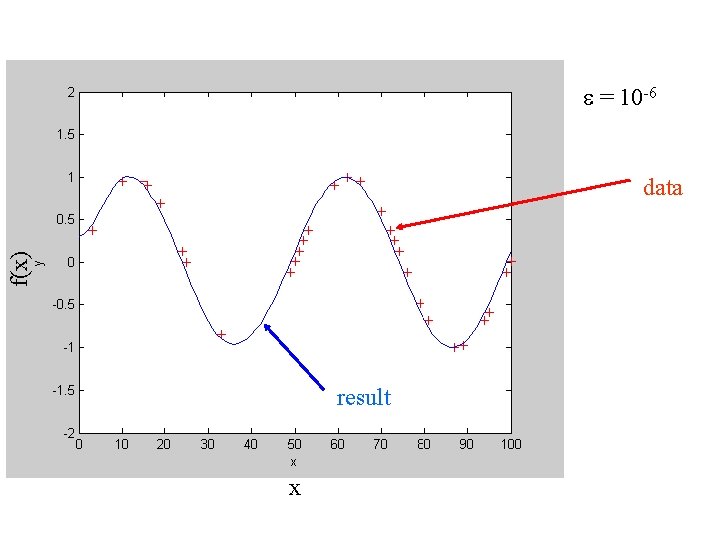
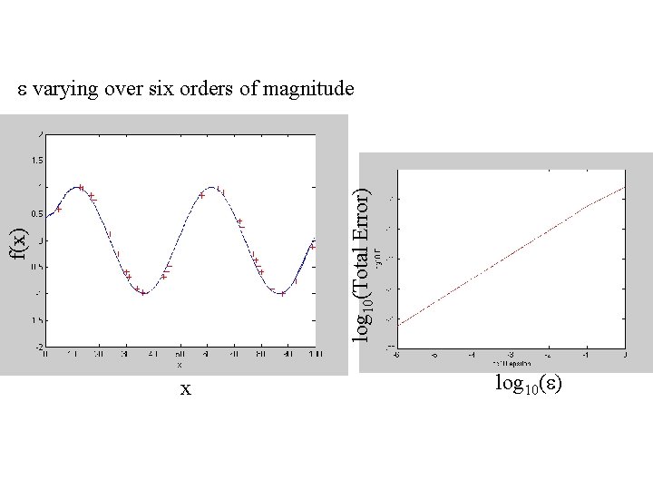
example 101 equally spaced along the x-axis So 101 values of the function f(x) 40 of these values measured (the data, d) the rest are unknown Two prior information minimize 2 nd derivative for interior 99 x’s minimize 1 st derivative at left and right x’s (nice to have the same number of priors as unknowns, but not required)

e = 10 -6 f(x) data result x

e can be chosen by trail and error but usually the result fairly insensitive to e, as long as its small

f(x) log 10(Total Error) e varying over six orders of magnitude x log 10(e)

A purist might say that this is not really interpolation, because the curve goes through the data only in the limit e 0 but for small e’s the error is extremely small

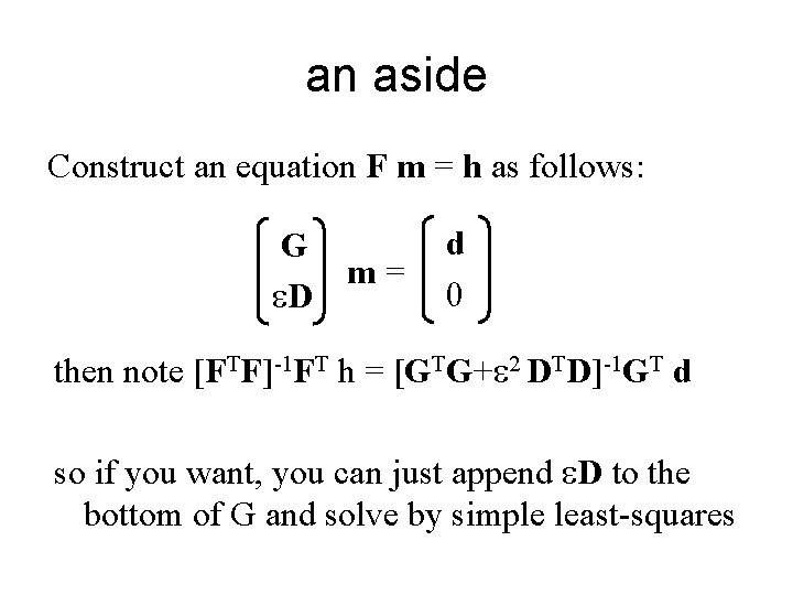
an aside Construct an equation F m = h as follows: G m= e. D d 0 then note [FTF]-1 FT h = [GTG+e 2 DTD]-1 GT d so if you want, you can just append e. D to the bottom of G and solve by simple least-squares

solved via [FTF]-1 FT h solved via [GTG+e 2 DTD]-1 GT d exactly the same!

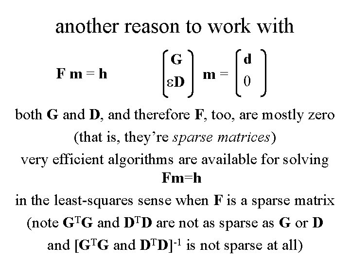
another reason to work with Fm=h G e. D d m= 0 both G and D, and therefore F, too, are mostly zero (that is, they’re sparse matrices) very efficient algorithms are available for solving Fm=h in the least-squares sense when F is a sparse matrix (note GTG and DTD are not as sparse as G or D and [GTG and DTD]-1 is not sparse at all)

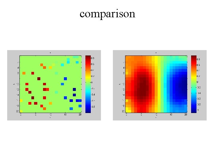
2 D Example (here a sparse solver would really be useful, for the number of unknowns is very large)

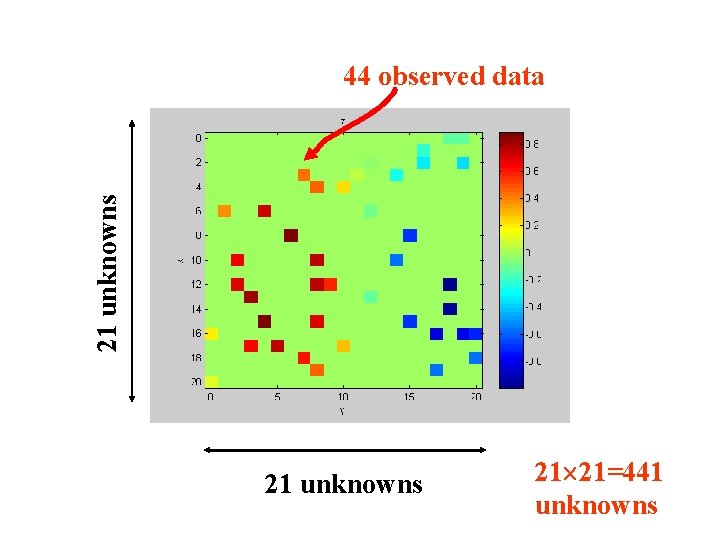
21 unknowns 44 observed data 21 unknowns 21 21=441 unknowns

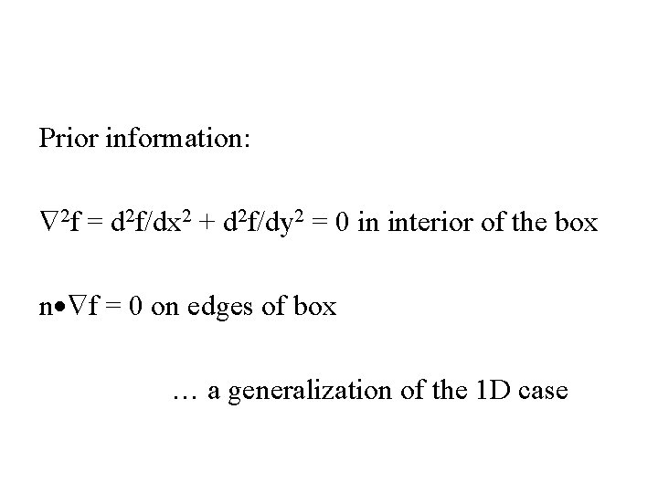
Prior information: 2 f = d 2 f/dx 2 + d 2 f/dy 2 = 0 in interior of the box n f = 0 on edges of box … a generalization of the 1 D case

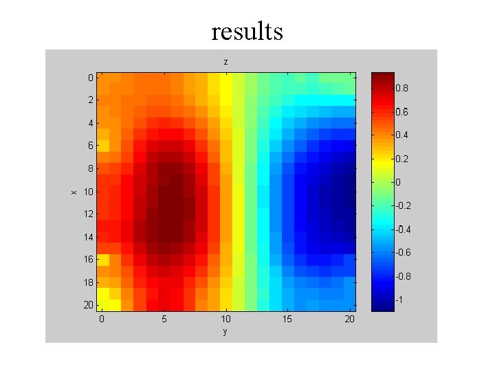
results

comparison

one limitation of this method is that it is discrete it only gives the unknown function at specific, prescribed values of xi one might prefer to have an analytic formula for the value of the function at any x

LINGO an analytic formula that gives the value of the function at any x is called an interpolant

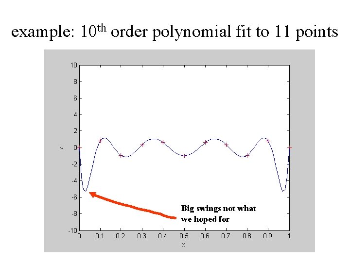
high order polynomial something that sound like a good idea but isn’t even though an N-1 polynomal can computed to pass through any N points

example: 10 th order polynomial fit to 11 points Big swings not what we hoped for

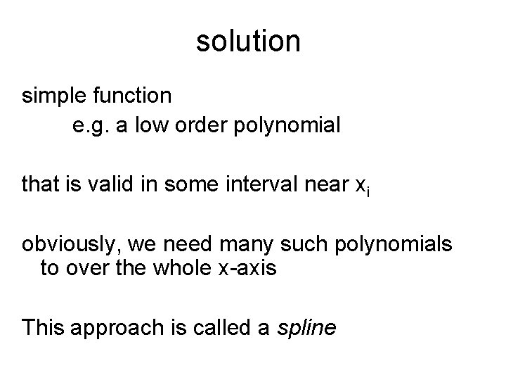
solution simple function e. g. a low order polynomial that is valid in some interval near xi obviously, we need many such polynomials to over the whole x-axis This approach is called a spline

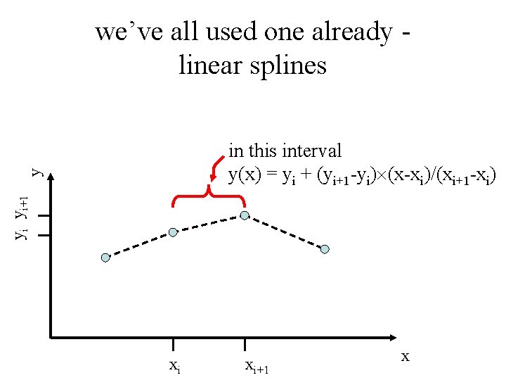
we’ve all used one already linear splines yi yi+1 y in this interval y(x) = yi + (yi+1 -yi) (x-xi)/(xi+1 -xi) xi xi+1 x

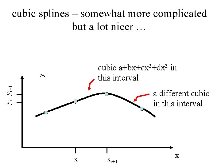
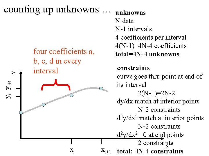
cubic splines – somewhat more complicated but a lot nicer … yi yi+1 y cubic a+bx+cx 2+dx 3 in this interval a different cubic in this interval xi xi+1 x

four coefficients a, b, c, d in every interval yi yi+1 y counting up unknowns … xi xi+1 unknowns N data N-1 intervals 4 coefficients per interval 4(N-1)=4 N-4 coefficients total=4 N-4 unknowns constraints curve goes thru point at end of its interval 2(N-1)=2 N-2 dy/dx match at interior points N-2 constraints d 2 y/dx 2 =0 at end points 2 constraints x total: 4 N-4 constraints

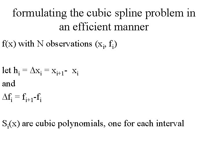
formulating the cubic spline problem in an efficient manner f(x) with N observations (xi, fi) let hi = Dxi = xi+1 - xi and Dfi = fi+1 -fi Si(x) are cubic polynomials, one for each interval

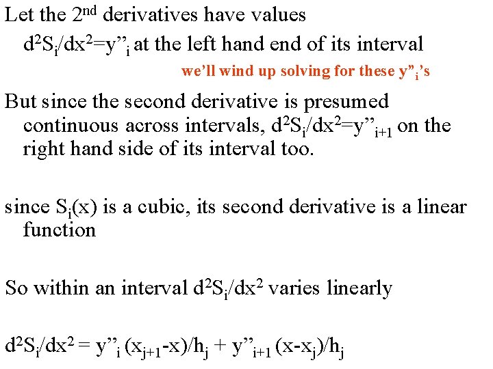
Let the 2 nd derivatives have values d 2 Si/dx 2=y”i at the left hand end of its interval we’ll wind up solving for these y”i’s But since the second derivative is presumed continuous across intervals, d 2 Si/dx 2=y”i+1 on the right hand side of its interval too. since Si(x) is a cubic, its second derivative is a linear function So within an interval d 2 Si/dx 2 varies linearly d 2 Si/dx 2 = y”i (xj+1 -x)/hj + y”i+1 (x-xj)/hj

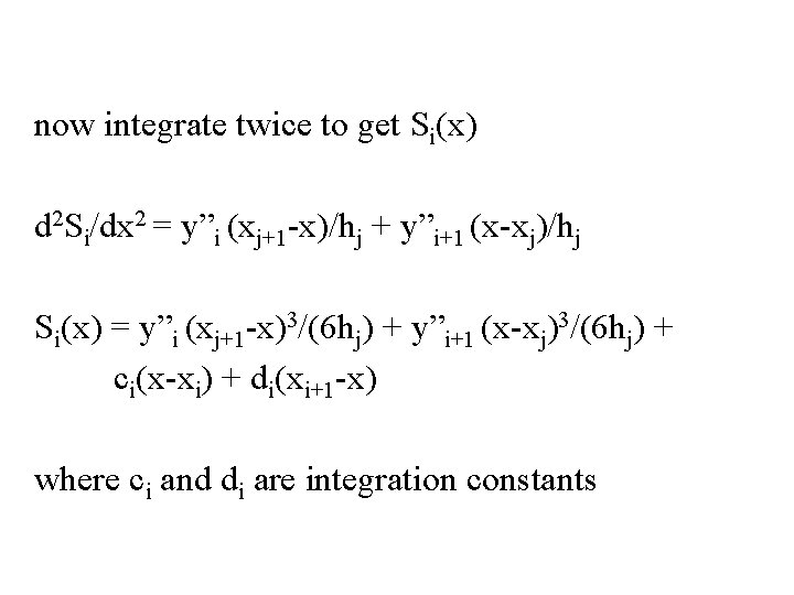
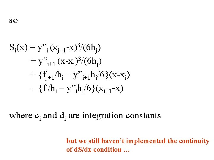
now integrate twice to get Si(x) d 2 Si/dx 2 = y”i (xj+1 -x)/hj + y”i+1 (x-xj)/hj Si(x) = y”i (xj+1 -x)3/(6 hj) + y”i+1 (x-xj)3/(6 hj) + ci(x-xi) + di(xi+1 -x) where ci and di are integration constants

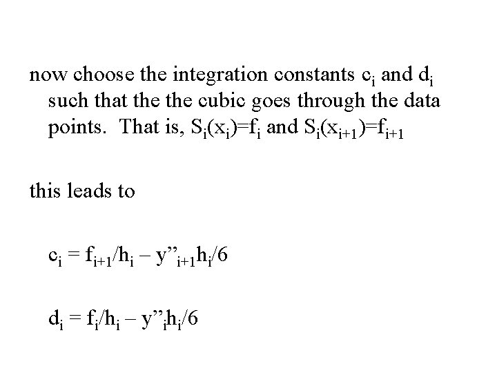
now choose the integration constants ci and di such that the cubic goes through the data points. That is, Si(xi)=fi and Si(xi+1)=fi+1 this leads to ci = fi+1/hi – y”i+1 hi/6 di = fi/hi – y”ihi/6

so Si(x) = y”i (xj+1 -x)3/(6 hj) + y”i+1 (x-xj)3/(6 hj) + {fj+1/hi – y”i+1 hi/6}(x-xi) + {fi/hi – y”ihi/6}(xi+1 -x) where ci and di are integration constants but we still haven’t implemented the continuity of d. S/dx condition …

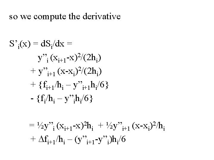
so we compute the derivative S’i(x) = d. Si/dx = y”i (xi+1 -x)2/(2 hi) + y”i+1 (x-xi)2/(2 hi) + {fi+1/hi – y”i+1 hi/6} - {fi/hi – y”ihi/6} = ½y”i (xi+1 -x)2 hi + ½y”i+1 (x-xi)2/hi + Dfi+1/hi – (y”i+1 -y”i)hi/6

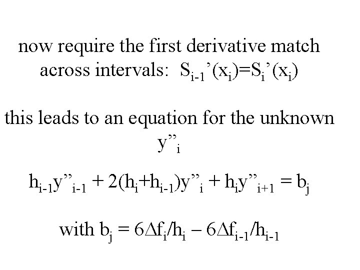
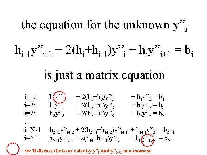
now require the first derivative match across intervals: Si-1’(xi)=Si’(xi) this leads to an equation for the unknown y”i hi-1 y”i-1 + 2(hi+hi-1)y”i + hiy”i+1 = bj with bj = 6 Dfi/hi – 6 Dfi-1/hi-1

the equation for the unknown y”i hi-1 y”i-1 + 2(hi+hi-1)y”i + hiy”i+1 = bi is just a matrix equation i=1: i=2: … i=N-1 i=N h 0 y” 0 h 1 y” 1 h 2 y” 2 + 2(h 1+h 0)y” 1 + 2(h 2+h 1)y” 2 + 2(h 3+h 2)y” 3 + h 1 y” 2 = b 1 + h 2 y” 2 = b 2 + h 3 y” 3 = b 3 h. N-2 y”N-2 + 2(h. N-1+h. N-2)y”N-1 + h. N-1 y”N = b. N-1 h. N-1 y”N-1 + 2(h. N+h. N-1)y”N + h. Ny”N+1 = b. N = we’ll discuss the issue raise by y” 0 and y”N+1 in a moment

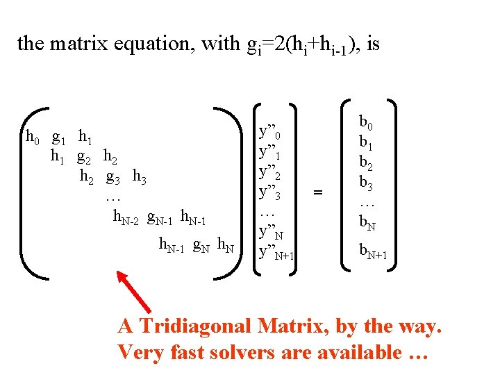
the matrix equation, with gi=2(hi+hi-1), is h 0 g 1 h 1 g 2 h 2 g 3 h 3 … h. N-2 g. N-1 h. N-1 g. N h. N y” 0 y” 1 y” 2 y” 3 … y”N+1 = b 0 b 1 b 2 b 3 … b. N+1 A Tridiagonal Matrix, by the way. Very fast solvers are available …

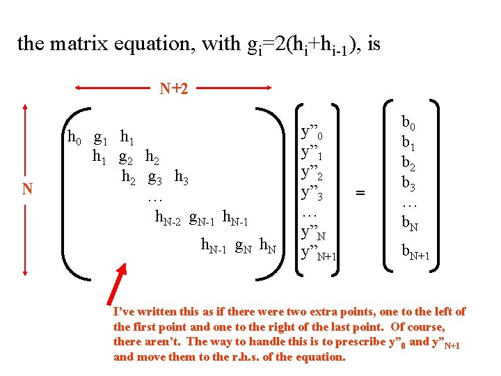
the matrix equation, with gi=2(hi+hi-1), is N+2 N h 0 g 1 h 1 g 2 h 2 g 3 h 3 … h. N-2 g. N-1 h. N-1 g. N h. N y” 0 y” 1 y” 2 y” 3 … y”N+1 = b 0 b 1 b 2 b 3 … b. N+1 I’ve written this as if there were two extra points, one to the left of the first point and one to the right of the last point. Of course, there aren’t. The way to handle this is to prescribe y” 0 and y”N+1 and move them to the r. h. s. of the equation.

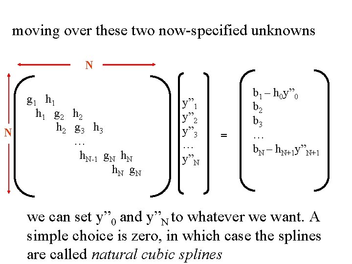
moving over these two now-specified unknowns N N g 1 h 1 g 2 h 2 g 3 h 3 … h. N-1 g. N h. N g. N y” 1 y” 2 y” 3 … y”N = b 1 – h 0 y” 0 b 2 b 3 … b. N – h. N+1 y”N+1 we can set y” 0 and y”N to whatever we want. A simple choice is zero, in which case the splines are called natural cubic splines

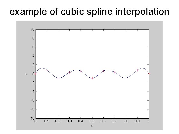
example of cubic spline interpolation

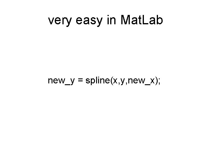
very easy in Mat. Lab new_y = spline(x, y, new_x);