INTERPOLATION Interpolation produces a function that matches the

INTERPOLATION Interpolation produces a function that matches the given data exactly. The function then can be utilized to approximate the data values at intermediate points.

Interpolation may also be used to produce a smooth graph of a function for which values are known only at discrete points, either from measurements or calculations.

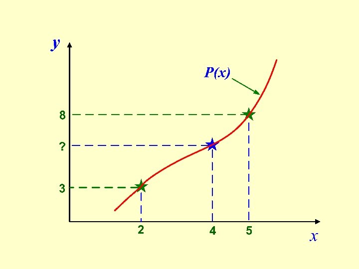
üGiven data points üObtain a function, P(x) üP(x) goes through the data points üUse P(x) üTo estimate values at intermediate points

Given data points: At x 0 = 2, y 0 = 3 and at x 1 = 5, y 1 = 8 Find the following: At x = 4, y = ?

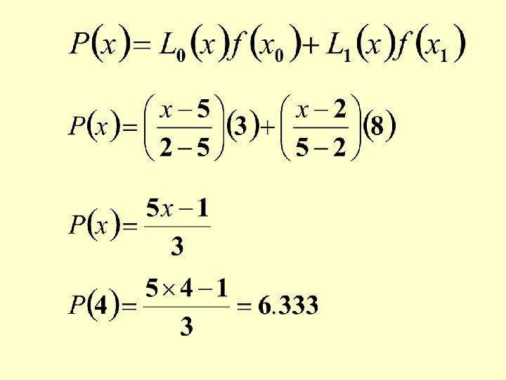
P(x) should satisfy the following conditions: P(x = 2) = 3 and P(x = 5) = 8 P(x) can satisfy the above conditions if at x = x 0 = 2, L 0(x) = 1 and L 1(x) = 0 and at x = x 1= 5, L 0(x) = 0 and L 1(x) = 1

At x = x 0 = 2, L 0(x) = 1 and L 1(x) = 0 and at x = x 1= 5, L 0(x) = 0 and L 1(x) = 1 The conditions can be satisfied if L 0(x) and L 1(x) are defined in the following way.

Lagrange Interpolating Polynomial

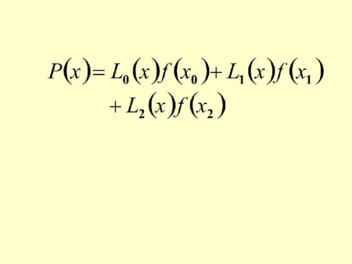
The Lagrange interpolating polynomial passing through three given points; (x 0, y 0), (x 1, y 1) and (x 2, y 2) is:

At x 0, L 0(x) becomes 1. At all other given data points L 0(x) is 0.

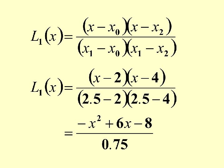
At x 1, L 1(x) becomes 1. At all other given data points L 1(x) is 0.

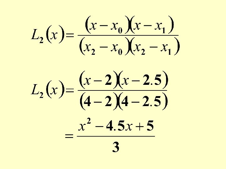
At x 2, L 2(x) becomes 1. At all other given data points L 2(x) is 0.

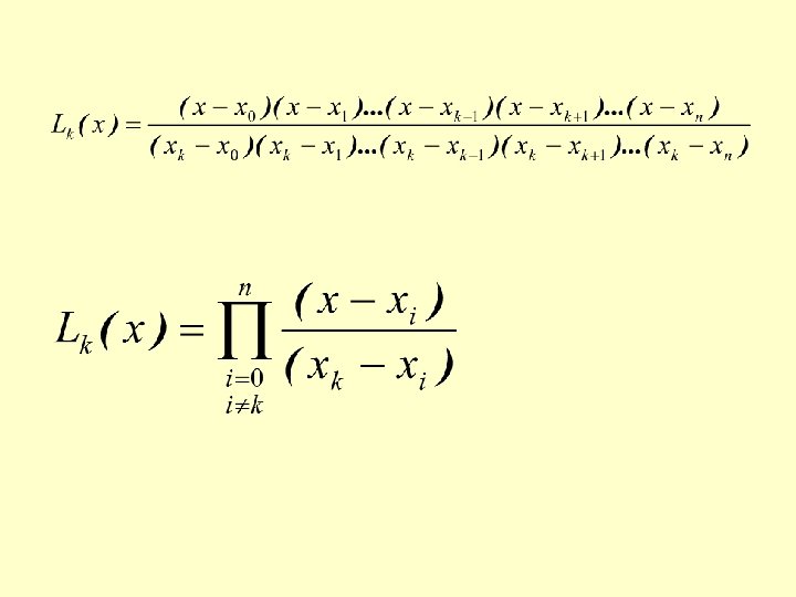
General form of the Lagrange Interpolating Polynomial

Numerator of

Denominator of

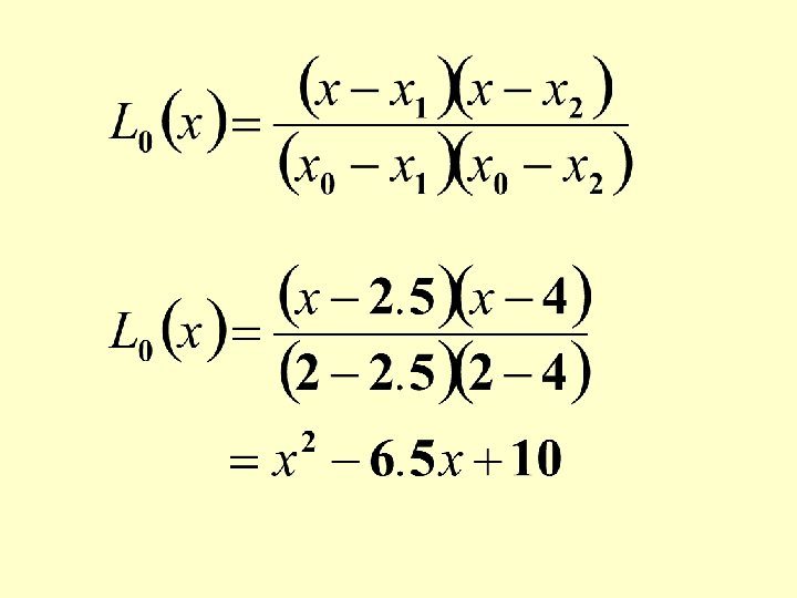
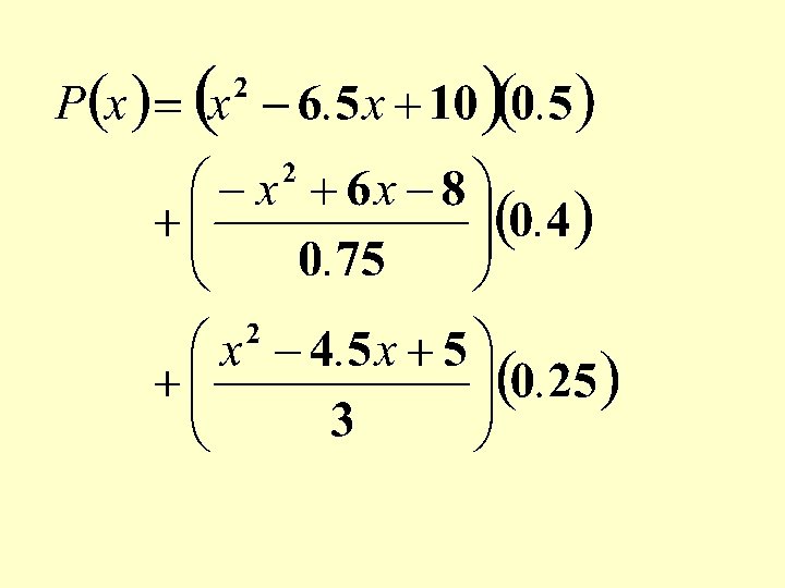
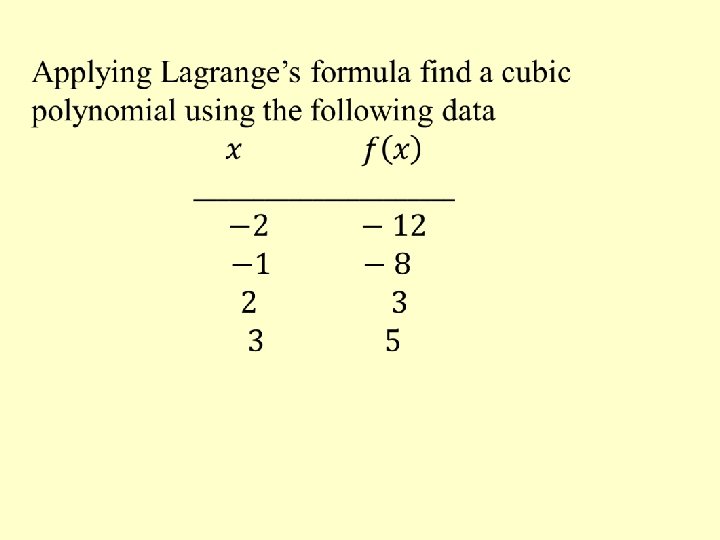
Find the Lagrange Interpolating Polynomial using the three given points.

The three given points were taken from the function

An approximation can be obtained from the Lagrange Interpolating Polynomial as:

• It is suspected that the high amounts of tannin in mature oak leave inhibit the growth of the winter moth larvae that extensively damage these trees in certain years. The following table lists the average weight of two samples of larvae at times in the first 28 days after birth. The first sample was reared on young oak leaves, whereas the second sample was reared on mature leaves from the same tree. • Use Lagrange’s interpolation to approximate the average weight curve for each sample. • Find an approximate maximum average weight for each sample by determining the maximum of the interpolating polynomial. Day 0 6 10 13 17 20 28 Sample 1 average weight(mg) 6. 67 17. 33 42. 67 37. 33 30. 10 29. 31 28. 74 Sample 2 average weight(mg) 6. 67 16. 11 18. 89 15. 00 10. 56 9. 44 8. 89

Newton’s Interpolating Polynomials Newton’s equation of a function that passes through two points and is

Set

Newton’s equation of a function that passes through three points and is

To find , set

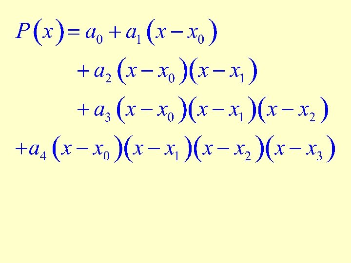
Newton’s equation of a function that passes through four points can be written by adding a fourth term.

The fourth term will vanish at all three previous points and, therefore, leaving all three previous coefficients intact.

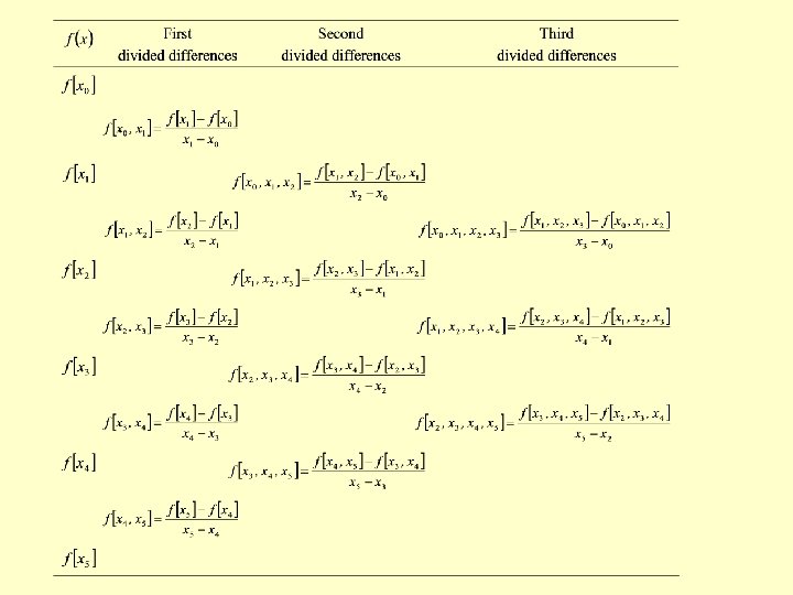
Divided differences and the coefficients The divided difference of a function, with respect to is denoted as It is called as zeroth divided difference and is simply the value of the function, at

The divided difference of a function, and with respect to called as the first divided difference, is denoted

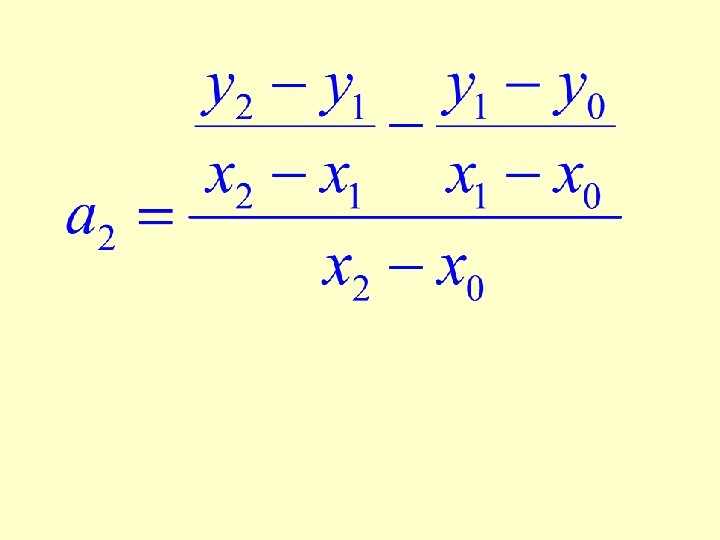
The divided difference of a function, , and with respect to called as the second divided difference, is denoted as

The third divided difference with respect to , , and

The coefficients of Newton’s interpolating polynomial are: and so on.

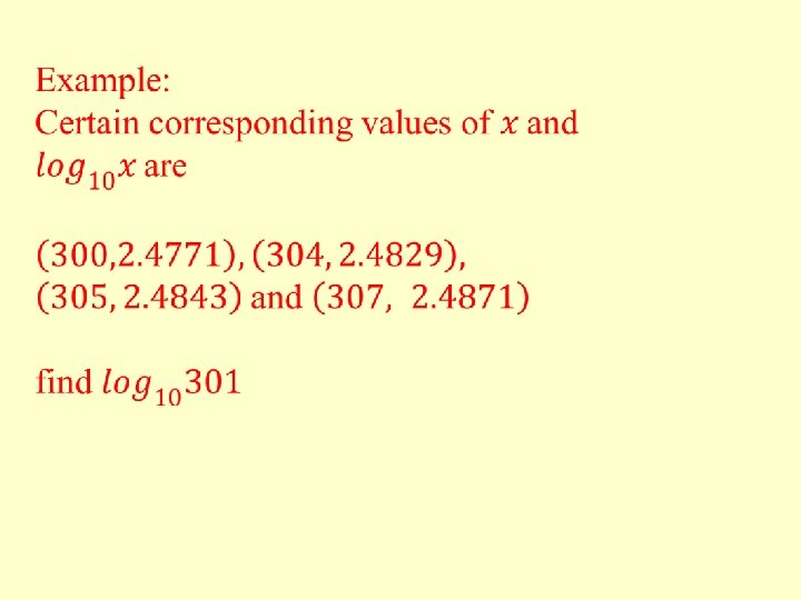
Example Find Newton’s interpolating polynomial to approximate a function whose 5 data points are given below. 2. 0 0. 85467 2. 3 0. 75682 2. 6 0. 43126 2. 9 0. 22364 3. 2 0. 08567

0 2. 0 0. 85467 -0. 32617 1 2. 3 0. 75682 -1. 26505 -1. 08520 2 2. 6 0. 43126 2. 13363 0. 65522 -0. 69207 3 2. 9 0. 22364 4 3. 2 0. 08567 -0. 29808 0. 38695 -0. 45990 -2. 02642

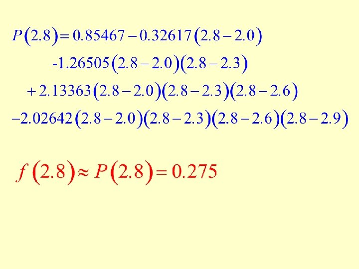
The 5 coefficients of the Newton’s interpolating polynomial are:

P(x) can now be used to estimate the value of the function f(x) say at x = 2. 8.

• Complete the divided difference table for the following data and also construct the interpolating polynomial that uses all this data. x f(x) 1. 0 0. 7651977 1. 3 0. 6200860 1. 6 0. 4554022 1. 9 0. 2818186 2. 2 0. 1103623