Interpolation Interpolation The process of inserting new data

Interpolation

Interpolation The process of inserting new data points between existing discrete data points Examples of Applications: 1. Signal Compression - some minimal amount data is stored or transmitted (enough to preserve the necessary information in the video or audio signal) then new data points are added when the signal is to be viewed (video) or listened to (audio) 2. Multi-rate Processing - altering the sampling rate of a digital signal in order to interface with a system operating at a different sampling rate 3. Estimation - estimating a value for a set of data when no data was collected (estimate the air temperature at 10: 15 am when data is collected every 10 minutes)

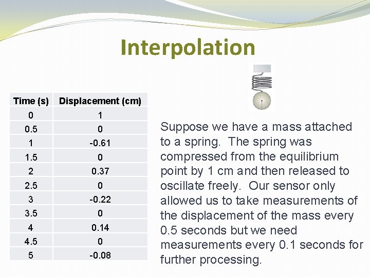
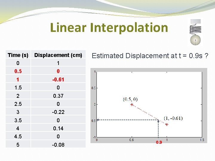
Interpolation Time (s) Displacement (cm) 0 1 0. 5 0 1 -0. 61 1. 5 0 2 0. 37 2. 5 0 3 -0. 22 3. 5 0 4 0. 14 4. 5 0 5 -0. 08 Suppose we have a mass attached to a spring. The spring was compressed from the equilibrium point by 1 cm and then released to oscillate freely. Our sensor only allowed us to take measurements of the displacement of the mass every 0. 5 seconds but we need measurements every 0. 1 seconds for further processing.

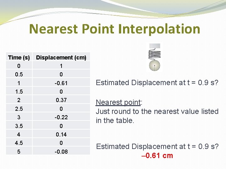
Nearest Point Interpolation Time (s) Displacement (cm) 0 1 0. 5 0 1 -0. 61 1. 5 0 2 0. 37 2. 5 0 3 -0. 22 3. 5 0 4 0. 14 4. 5 0 5 -0. 08 Estimated Displacement at t = 0. 9 s? Nearest point: Just round to the nearest value listed in the table. Estimated Displacement at t = 0. 9 s? -0. 61 cm

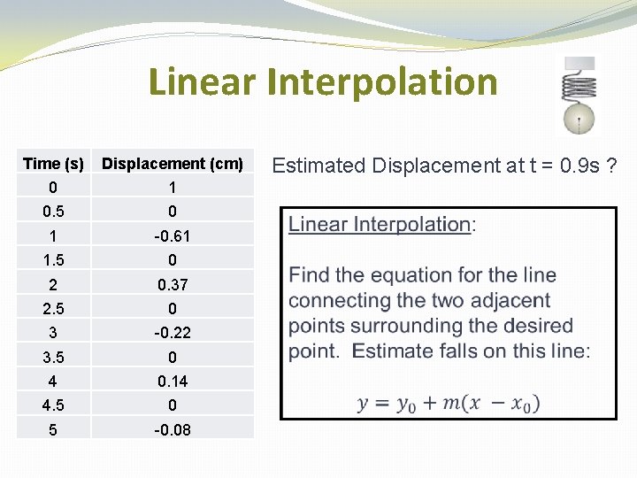
Linear Interpolation Time (s) Displacement (cm) 0 1 0. 5 0 1 -0. 61 1. 5 0 2 0. 37 2. 5 0 3 -0. 22 3. 5 0 4 0. 14 4. 5 0 5 -0. 08 Estimated Displacement at t = 0. 9 s ?

Linear Interpolation Time (s) Displacement (cm) 0 1 0. 5 0 1 -0. 61 1. 5 0 2 0. 37 2. 5 0 3 -0. 22 3. 5 0 4 0. 14 4. 5 0 5 -0. 08 Estimated Displacement at t = 0. 9 s ? 0. 9

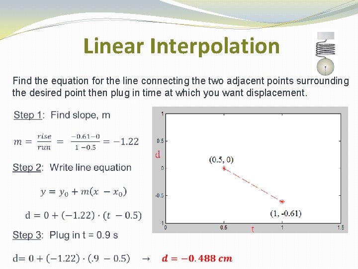
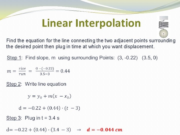
Linear Interpolation Find the equation for the line connecting the two adjacent points surrounding the desired point then plug in time at which you want displacement.

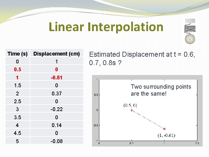
Linear Interpolation Time (s) Displacement (cm) 0 1 0. 5 0 1 -0. 61 1. 5 0 2 0. 37 2. 5 0 3 -0. 22 3. 5 0 4 0. 14 4. 5 0 5 -0. 08 Estimated Displacement at t = 0. 6, 0. 7, 0. 8 s ? Two surrounding points are the same!

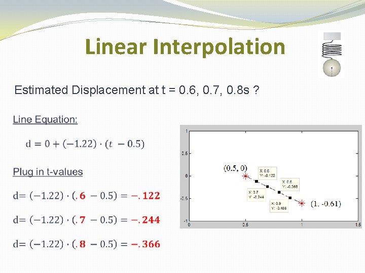
Linear Interpolation Estimated Displacement at t = 0. 6, 0. 7, 0. 8 s ?

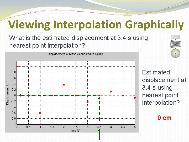
Viewing Interpolation Graphically What is the estimated displacement at 3. 4 s using nearest point interpolation? Estimated displacement at 3. 4 s using nearest point interpolation? 0 cm

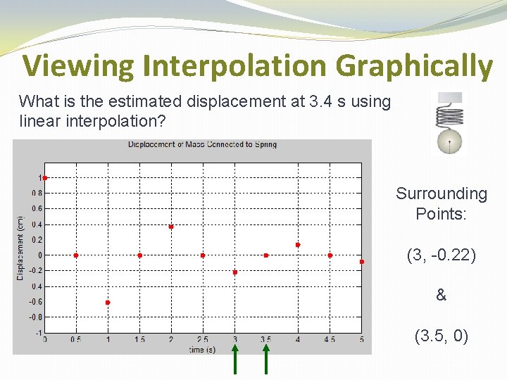
Viewing Interpolation Graphically What is the estimated displacement at 3. 4 s using linear interpolation? Surrounding Points: (3, -0. 22) & (3. 5, 0)

Linear Interpolation Find the equation for the line connecting the two adjacent points surrounding the desired point then plug in time at which you want displacement.

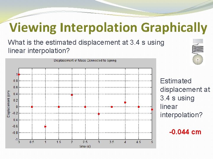
Viewing Interpolation Graphically What is the estimated displacement at 3. 4 s using linear interpolation? Estimated displacement at 3. 4 s using linear interpolation? -0. 044 cm

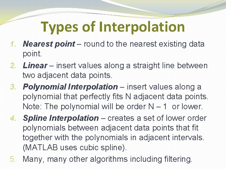
Types of Interpolation 1. Nearest point – round to the nearest existing data point. 2. Linear – insert values along a straight line between two adjacent data points. 3. Polynomial Interpolation – insert values along a polynomial that perfectly fits N adjacent data points. Note: The polynomial will be order N – 1 or lower. 4. Spline Interpolation – creates a set of lower order polynomials between adjacent data points that fit together with the polynomials in adjacent intervals. (MATLAB uses cubic spline). 5. Many, many other algorithms including filtering.

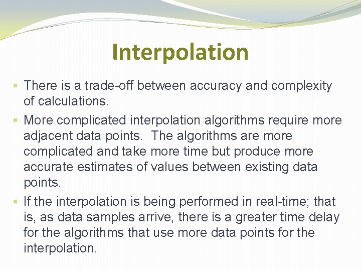
Interpolation § There is a trade-off between accuracy and complexity of calculations. § More complicated interpolation algorithms require more adjacent data points. The algorithms are more complicated and take more time but produce more accurate estimates of values between existing data points. § If the interpolation is being performed in real-time; that is, as data samples arrive, there is a greater time delay for the algorithms that use more data points for the interpolation.

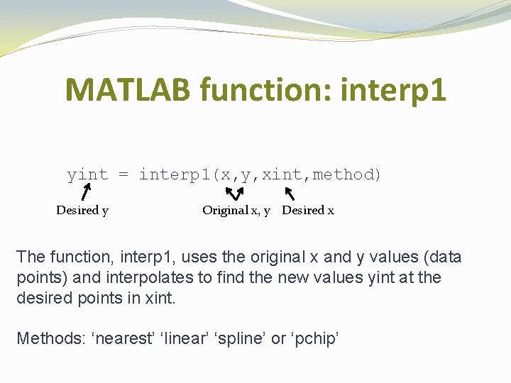
MATLAB function: interp 1 yint = interp 1(x, y, xint, method) Desired y Original x, y Desired x The function, interp 1, uses the original x and y values (data points) and interpolates to find the new values yint at the desired points in xint. Methods: ‘nearest’ ‘linear’ ‘spline’ or ‘pchip’

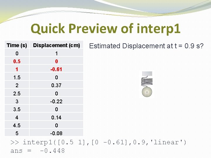
Quick Preview of interp 1 Time (s) Displacement (cm) 0 1 0. 5 0 1 -0. 61 1. 5 0 2 0. 37 2. 5 0 3 -0. 22 3. 5 0 4 0. 14 4. 5 0 5 -0. 08 Estimated Displacement at t = 0. 9 s? >> interp 1([0. 5 1], [0 -0. 61], 0. 9, 'linear') ans = -0. 448

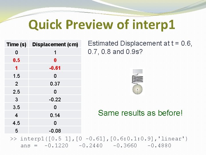
Quick Preview of interp 1 Time (s) Displacement (cm) 0 1 0. 5 0 1 -0. 61 1. 5 0 2 0. 37 2. 5 0 3 -0. 22 3. 5 0 4 0. 14 4. 5 0 5 -0. 08 Estimated Displacement at t = 0. 6, 0. 7, 0. 8 and 0. 9 s? Same results as before! >> interp 1([0. 5 1], [0 -0. 61], [0. 6: 0. 1: 0. 9], 'linear') ans = -0. 1220 -0. 2440 -0. 3660 -0. 4880

Interpolation vs. Curve Fitting �Interpolation stuffs new data points between existing points without attempting to determine some overall mathematical expression. Interpolation utilizes equations that are satisfied by the subset of existing data points being used for the interpolation calculation. Existing data points are not modified. �Curve fitting does not require that any of the existing data points satisfy the resulting mathematical expression. It is possible that none of the original data points are on the graph of the resulting function.

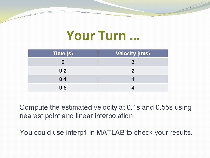
Your Turn … Time (s) Velocity (m/s) 0 3 0. 2 2 0. 4 1 0. 6 4 Compute the estimated velocity at 0. 1 s and 0. 55 s using nearest point and linear interpolation. You could use interp 1 in MATLAB to check your results.

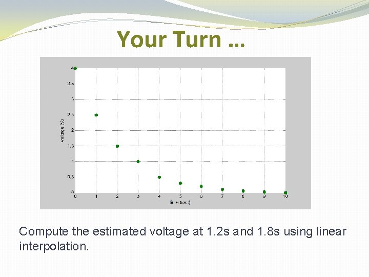
Your Turn … Compute the estimated voltage at 1. 2 s and 1. 8 s using linear interpolation.

Test Your Understanding