The simulation of droplets bubbles and interfaces Stphane

The simulation of droplets, bubbles and interfaces Stéphane Zaleski Institut Jean Le Rond ∂’Alembert, Université Pierre et Marie Curie UPMC – Paris 6 1/61

Simulation of multiphase flows progresses at an amazing rate 2/61

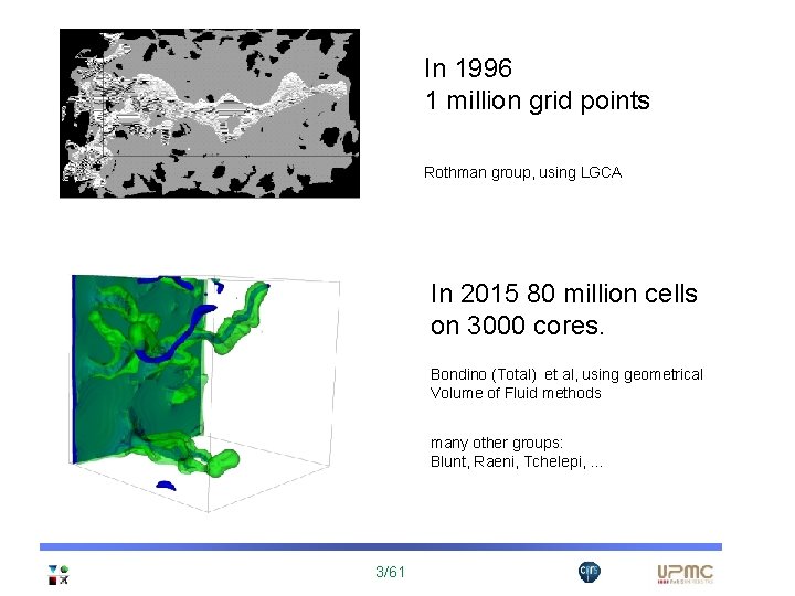
In 1996 1 million grid points Rothman group, using LGCA In 2015 80 million cells on 3000 cores. Bondino (Total) et al, using geometrical Volume of Fluid methods many other groups: Blunt, Raeni, Tchelepi, . . . 3/61

The progress for open flows such as atomization is even more spectular 4/61

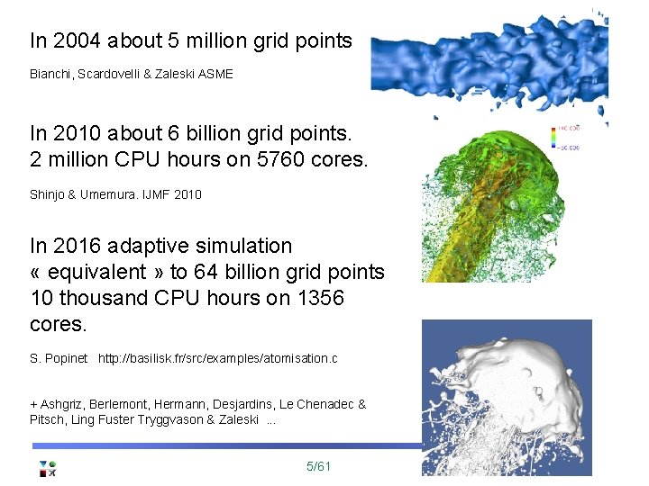
In 2004 about 5 million grid points Bianchi, Scardovelli & Zaleski ASME In 2010 about 6 billion grid points. 2 million CPU hours on 5760 cores. Shinjo & Umemura. IJMF 2010 In 2016 adaptive simulation « equivalent » to 64 billion grid points 10 thousand CPU hours on 1356 cores. S. Popinet http: //basilisk. fr/src/examples/atomisation. c + Ashgriz, Berlemont, Hermann, Desjardins, Le Chenadec & Pitsch, Ling Fuster Tryggvason & Zaleski . . . 5/61

Why is progress faster on atomization than on porous media simulation ? Are the problems intrinsically harder ? Raw speed is not the only characteristic of codes. 6/61

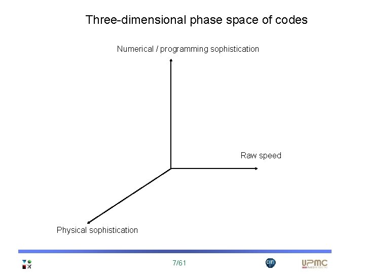
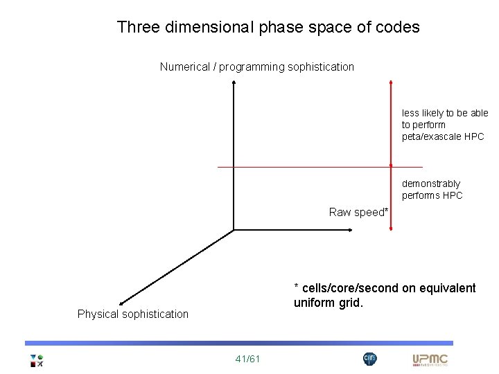
Three-dimensional phase space of codes Numerical / programming sophistication Raw speed Physical sophistication 7/61

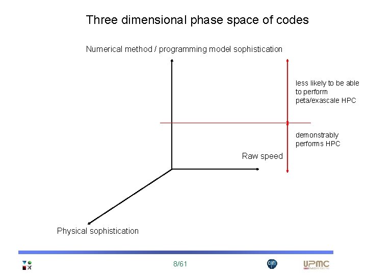
Three dimensional phase space of codes Numerical method / programming model sophistication less likely to be able to perform peta/exascale HPC demonstrably performs HPC Raw speed Physical sophistication 8/61

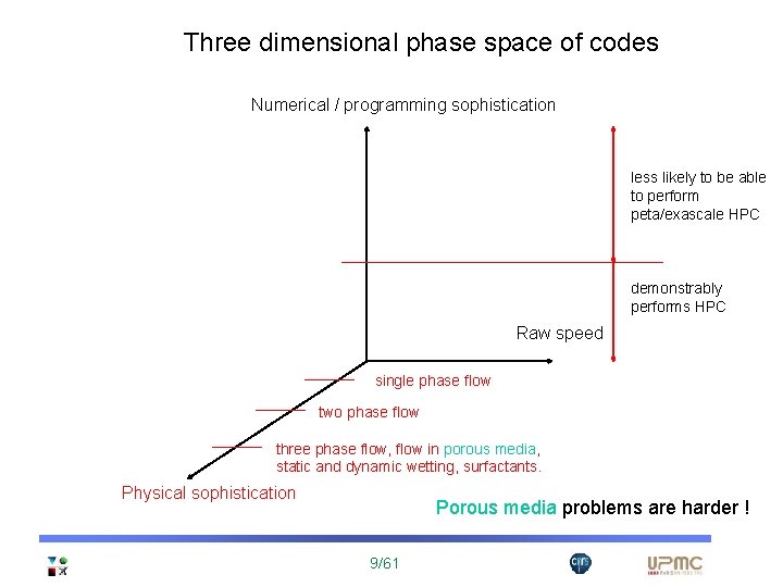
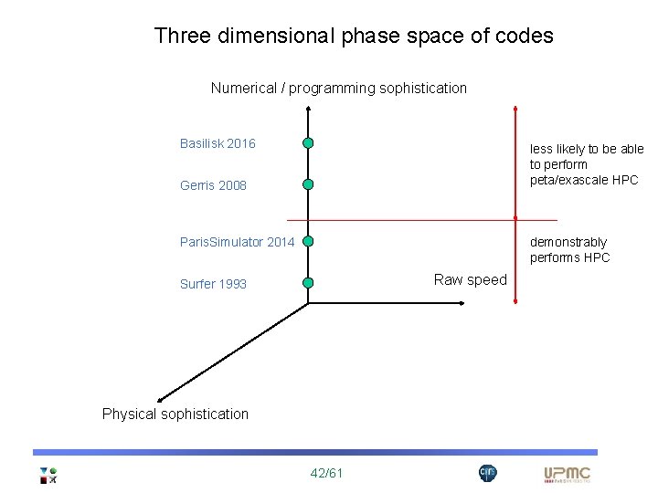
Three dimensional phase space of codes Numerical / programming sophistication less likely to be able to perform peta/exascale HPC demonstrably performs HPC Raw speed single phase flow two phase flow three phase flow, flow in porous media, static and dynamic wetting, surfactants. Physical sophistication Porous media problems are harder ! 9/61

In what follows, I will mostly talk about : 1. Numerical methods for two phase flows 2. Results on some physical problems 3. To a lesser extent, codes. 1. How to model & simulate multiphase flows ? 10/61

1. How to model & simulate multiphase flows ? - 1 Compute an evolving surface : computational geometry - Solve 2 the Navier-Stokes or Stokes equations with 3 surface tension and 4 variable viscosity and density 11/61

1. Compute surface evolution it is a kind of computational geometry Why is it difficult to follow evolving surfaces ? - geometrical complexity (curved surfaces, how they cut – change topology) - numerical stability issues of the most obvious methods. - accuracy issues (high accuracy is needed: surface tension effects depend on the third derivative of the interface position. ) 12/61

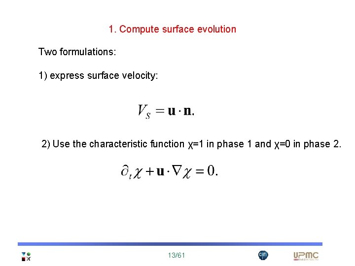
1. Compute surface evolution Two formulations: 1) express surface velocity: 2) Use the characteristic function χ=1 in phase 1 and χ=0 in phase 2. 13/61

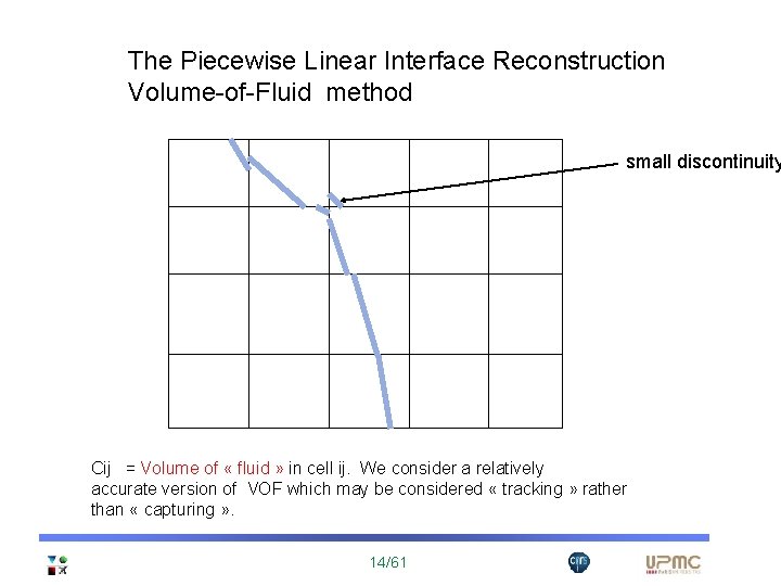
The Piecewise Linear Interface Reconstruction Volume-of-Fluid method small discontinuity Cij = Volume of « fluid » in cell ij. We consider a relatively accurate version of VOF which may be considered « tracking » rather than « capturing » . 14/61

Two kinds of VOF methods: - « off the shelf » methods for hyperbolic PDE / gas dynamics. (Open. Foam, JADIM etc. . ) - methods involving geometric operations (Surfer, Gerris, Basilisk, Paris. Simulator) 15/61

Reconstruction in 3 D - compute interface normal n - place interface segment once interface normal is known 12 critical cases in 3 D for all ni > 0 16/61

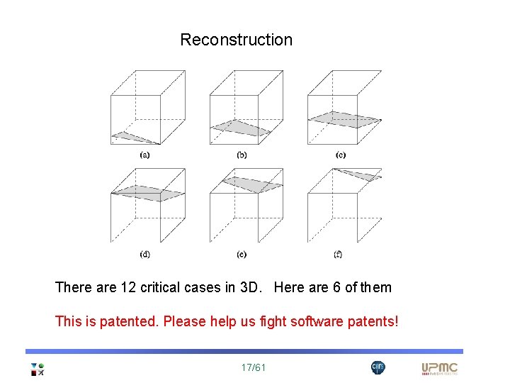
Reconstruction There are 12 critical cases in 3 D. Here are 6 of them This is patented. Please help us fight software patents! 17/61

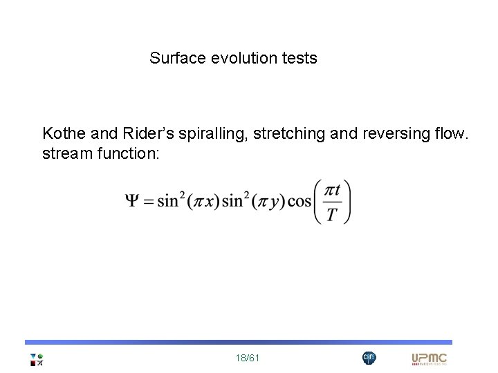
Surface evolution tests Kothe and Rider’s spiralling, stretching and reversing flow. stream function: 18/61

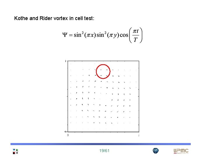
Kothe and Rider vortex in cell test: 19/61

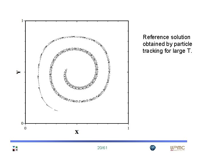
Reference solution obtained by particle tracking for large T. 20/61

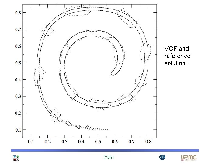
VOF and reference solution. 21/61

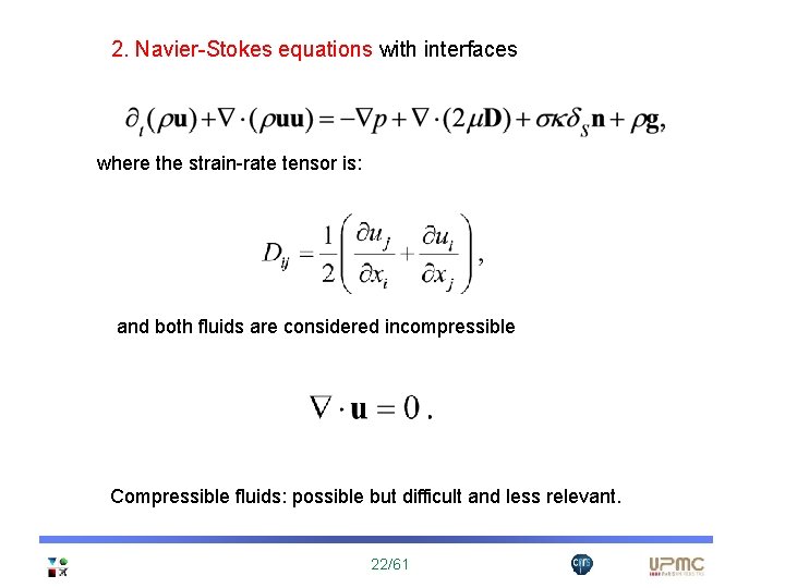
2. Navier-Stokes equations with interfaces where the strain-rate tensor is: and both fluids are considered incompressible Compressible fluids: possible but difficult and less relevant. 22/61

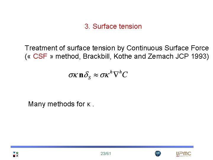
3. Surface tension Treatment of surface tension by Continuous Surface Force ( « CSF » method, Brackbill, Kothe and Zemach JCP 1993) Many methods for κ. 23/61

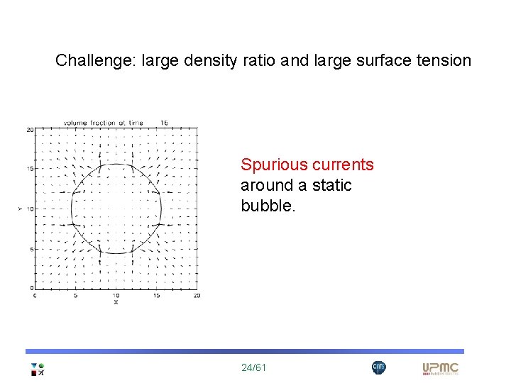
Challenge: large density ratio and large surface tension Spurious currents around a static bubble. 24/61

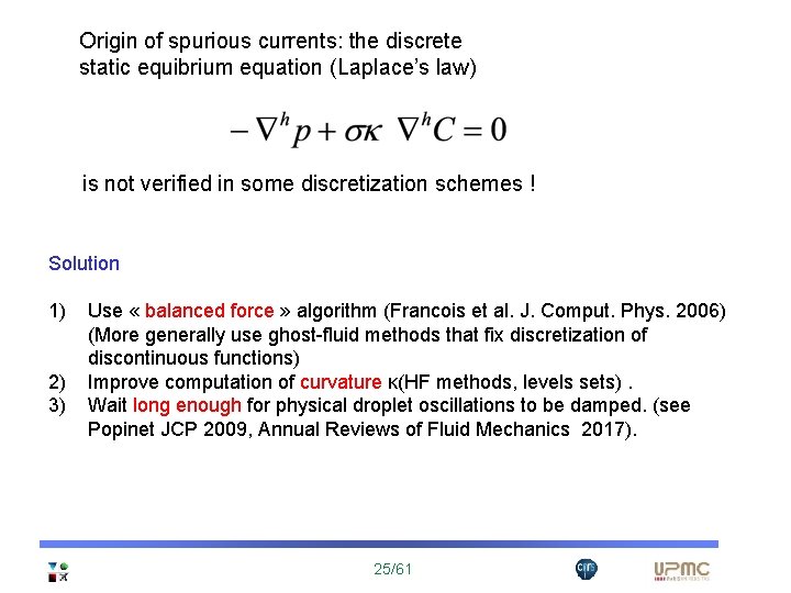
Origin of spurious currents: the discrete static equibrium equation (Laplace’s law) is not verified in some discretization schemes ! Solution 1) 2) 3) Use « balanced force » algorithm (Francois et al. J. Comput. Phys. 2006) (More generally use ghost-fluid methods that fix discretization of discontinuous functions) Improve computation of curvature κ(HF methods, levels sets). Wait long enough for physical droplet oscillations to be damped. (see Popinet JCP 2009, Annual Reviews of Fluid Mechanics 2017). 25/61

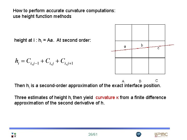
How to perform accurate curvature computations: use height function methods height at i : hi = Aa. At second order: Then hi is a second-order approximation of the exact interface position. Three estimates of height hi then yield curvature κ from a finite difference approximation of the second derivative of h. 26/61

4. Variable viscosity - Two possibilities in mixed cells: arithmetic mean or harmonic mean - The harmonic mean is exact for a linear, parallel shear flow. 27/61

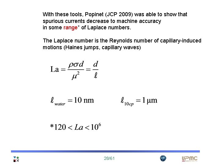
With these tools, Popinet (JCP 2009) was able to show that spurious currents decrease to machine accuracy in some range* of Laplace numbers. The Laplace number is the Reynolds number of capillary-induced motions (Haines jumps, capillary waves) 28/61

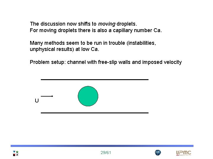
The discussion now shifts to moving droplets. For moving droplets there is also a capillary number Ca. Many methods seem to be run in trouble (instabilities, unphysical results) at low Ca. Problem setup: channel with free-slip walls and imposed velocity U 29/61

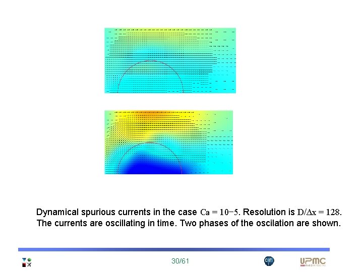
Dynamical spurious currents in the case Ca = 10− 5. Resolution is D/∆x = 128. The currents are oscillating in time. Two phases of the oscilation are shown. 30/61

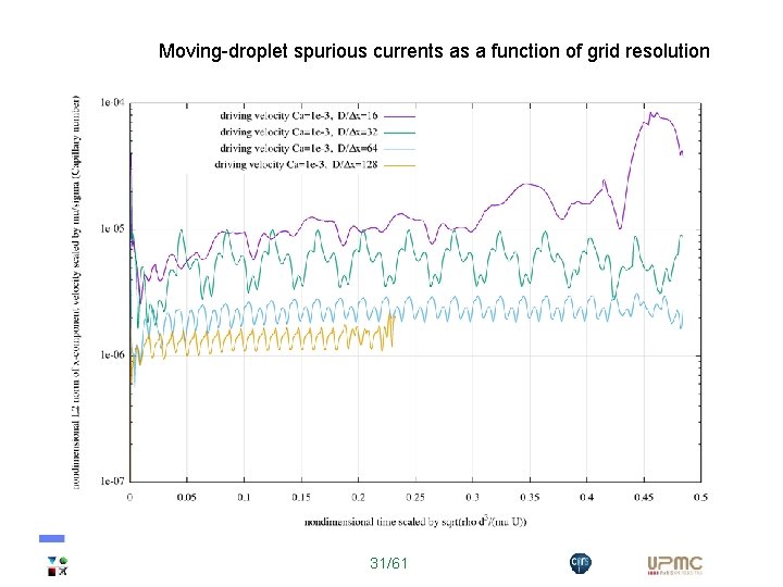
Moving-droplet spurious currents as a function of grid resolution 31/61

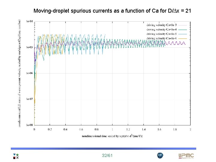
Moving-droplet spurious currents as a function of Ca for D/∆x = 21 32/61

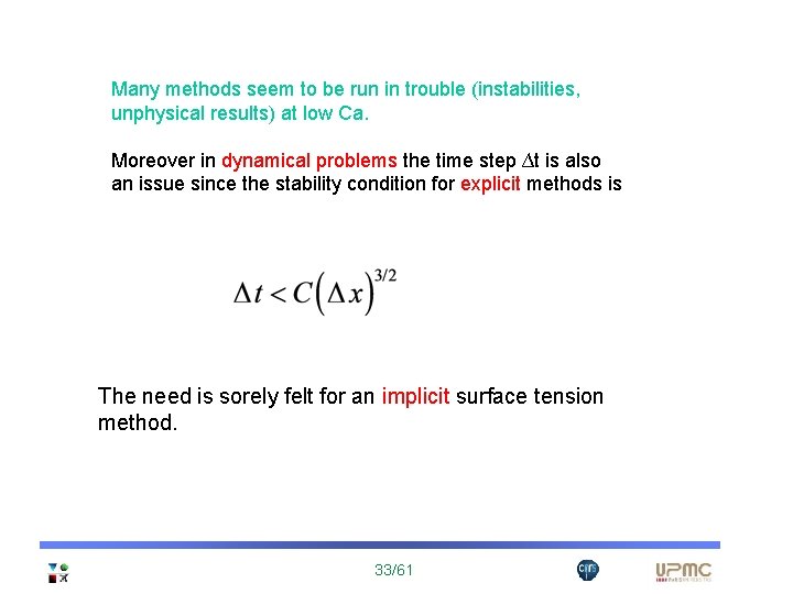
Many methods seem to be run in trouble (instabilities, unphysical results) at low Ca. Moreover in dynamical problems the time step ∆t is also an issue since the stability condition for explicit methods is The need is sorely felt for an implicit surface tension method. 33/61

Implementation of VOF methods in several codes: Surfer, Gerris, Open. Foam, Parissimulator, Basilisk etc. . . (all free) 34/61

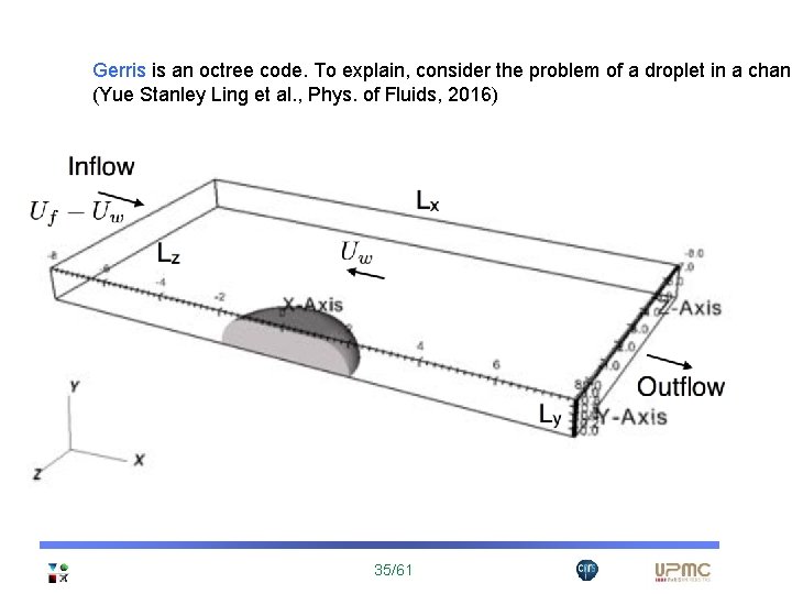
Gerris is an octree code. To explain, consider the problem of a droplet in a chann (Yue Stanley Ling et al. , Phys. of Fluids, 2016) 35/61

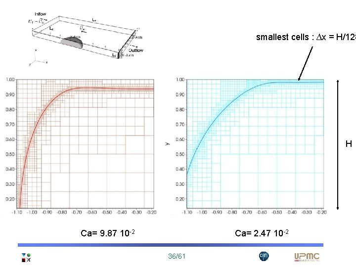
smallest cells : ∆x = H/128 H Ca= 9. 87 10 -2 Ca= 2. 47 10 -2 36/61

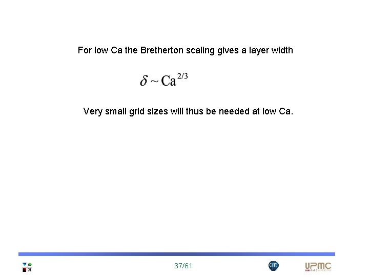
For low Ca the Bretherton scaling gives a layer width Very small grid sizes will thus be needed at low Ca. 37/61

Attempts at more complex simulations 38/61

We attempted an invasion simulation with Gerris (Bondino, Lagrée SIAM 2014) but it is: - slow - the code is buggy - the code does not parallelize properly Challenge: do better. Two approaches: 1) a much more efficient approach to computing on octree: Basilisk by S. Popinet: http: //basilisk. fr 2) or a very simple code on regular grids: Paris. Simulator by Scardovelli, Ling, Tryggvason, Zaleski http: //parissimulator. sf. net 39/61

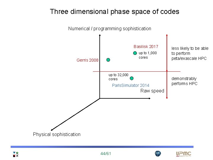
the Paris. Simulator code - Multimethod code with VOF and Front Tracking (In what follows we use only VOF) - Exactly mass-conserving option. - Exactly momentum-conserving option. - Written in Fortran 95 -2002 - Regular grid, excellent parallelisation tested up to 32, 000 cores. - Free code. 40/61

Three dimensional phase space of codes Numerical / programming sophistication less likely to be able to perform peta/exascale HPC demonstrably performs HPC Raw speed* * cells/core/second on equivalent uniform grid. Physical sophistication 41/61

Three dimensional phase space of codes Numerical / programming sophistication Basilisk 2016 less likely to be able to perform peta/exascale HPC Gerris 2008 Paris. Simulator 2014 demonstrably performs HPC Raw speed Surfer 1993 Physical sophistication 42/61

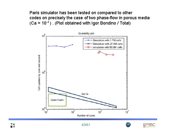
Paris simulator has been tested on compared to other codes on precisely the case of two phase-flow in porous media (Ca = 10 -4 ). (Plot obtained with Igor Bondino / Total) 43/61

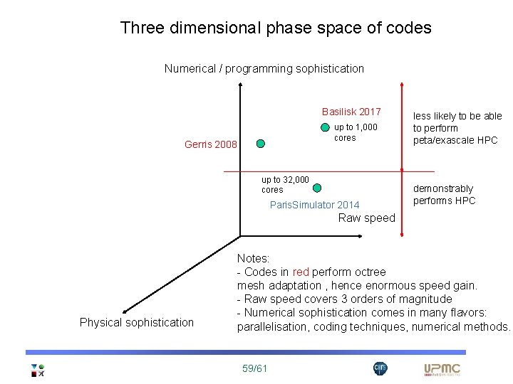
Three dimensional phase space of codes Numerical / programming sophistication Basilisk 2017 up to 1, 000 cores Gerris 2008 up to 32, 000 cores Paris. Simulator 2014 Raw speed Physical sophistication 44/61 less likely to be able to perform peta/exascale HPC demonstrably performs HPC

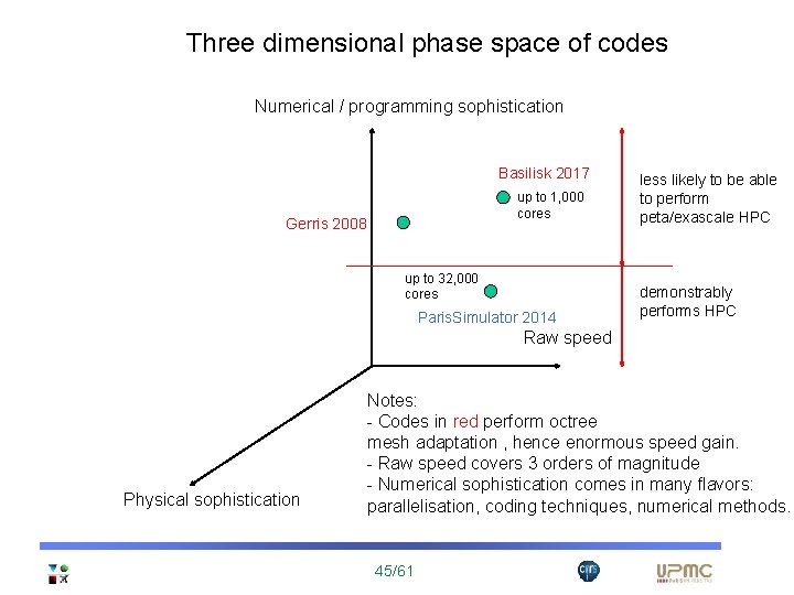
Three dimensional phase space of codes Numerical / programming sophistication Basilisk 2017 up to 1, 000 cores Gerris 2008 up to 32, 000 cores Paris. Simulator 2014 less likely to be able to perform peta/exascale HPC demonstrably performs HPC Raw speed Physical sophistication Notes: - Codes in red perform octree mesh adaptation , hence enormous speed gain. - Raw speed covers 3 orders of magnitude - Numerical sophistication comes in many flavors: parallelisation, coding techniques, numerical methods. 45/61

2. Results 46/61

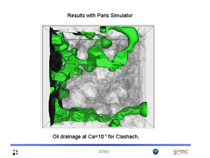
Results with Paris Simulator Oil drainage at Ca=10 -4 for Clashach, 47/61

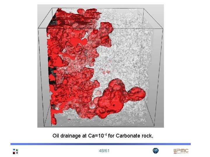
Oil drainage at Ca=10 -4 for Carbonate rock, 48/61

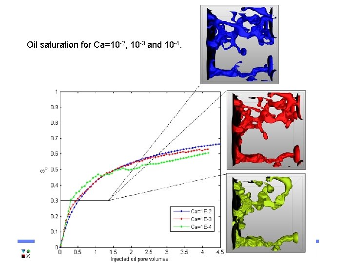
Oil saturation for Ca=10 -2, 10 -3 and 10 -4. 49/61

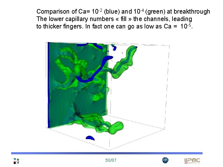
Comparison of Ca= 10 -2 (blue) and 10 -4 (green) at breakthrough The lower capillary numbers « fill » the channels, leading to thicker fingers. In fact one can go as low as Ca = 10 -5. 50/87

We used the simulation to estimate the permeabilities using both a global method and a local method. • In the local method (M 1) the rock is split in several slices perpendicular to the injection flow. • In the global method (M 2) we apply the relative permeability concept over the entire model rock sample. 51/61

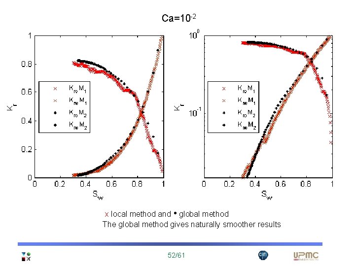
Ca=10 -2 x local method and • global method The global method gives naturally smoother results 52/61

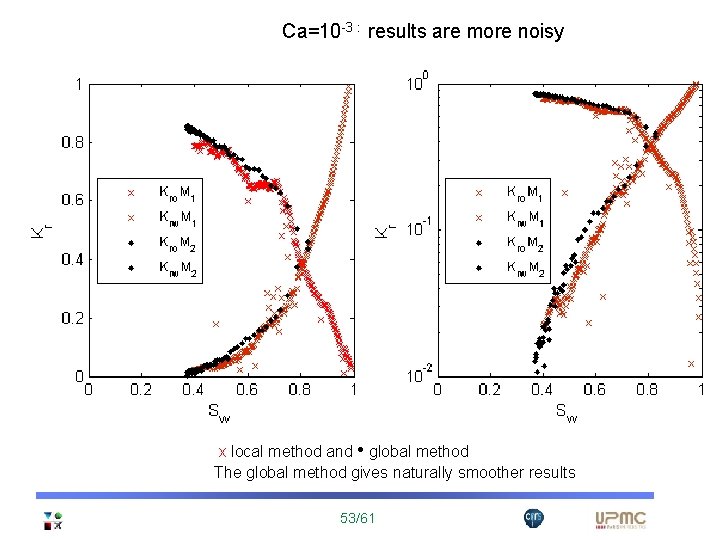
Ca=10 -3 : results are more noisy x local method and • global method The global method gives naturally smoother results 53/61

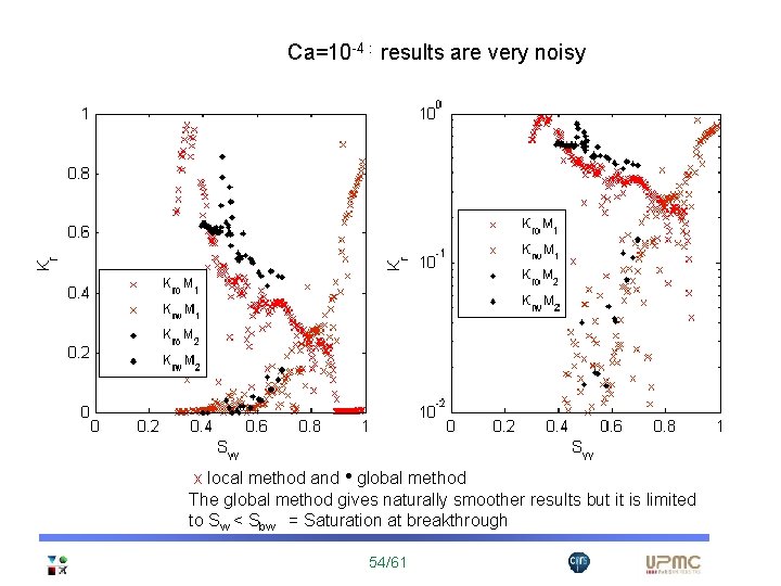
Ca=10 -4 : results are very noisy x local method and • global method The global method gives naturally smoother results but it is limited to Sw < Sbw = Saturation at breakthrough 54/61

Beyond Gerris: basilisk 55/61

Parellisation and Octree: new « basilisk » code by Stéphane Popinet. Example: CORIA – Berlemont jet, Resolution 40963 on 1536 cores ~ 104 hours (less than 5 hours wall clock time ! 56/61

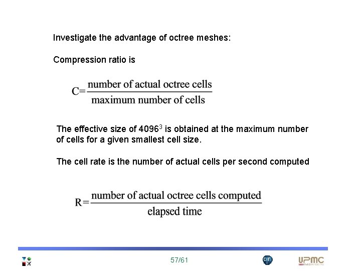
Investigate the advantage of octree meshes: Compression ratio is The effective size of 40963 is obtained at the maximum number of cells for a given smallest cell size. The cell rate is the number of actual cells per second computed 57/61

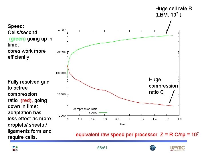
Huge cell rate R (LBM: 107 ) Speed: Cells/second (green) going up in time: cores work more efficiently Fully resolved grid to octree compression ratio (red), going down in time: adaptation has less effect as more droplets/ sheets / ligaments form and require cells. Huge compression ratio C equivalent raw speed per processor Z = R C/np = 107 58/61

Three dimensional phase space of codes Numerical / programming sophistication Basilisk 2017 up to 1, 000 cores Gerris 2008 up to 32, 000 cores Paris. Simulator 2014 less likely to be able to perform peta/exascale HPC demonstrably performs HPC Raw speed Physical sophistication Notes: - Codes in red perform octree mesh adaptation , hence enormous speed gain. - Raw speed covers 3 orders of magnitude - Numerical sophistication comes in many flavors: parallelisation, coding techniques, numerical methods. 59/61

Perspectives: - « hyperachiever » codes and methods combining complexity and efficiency - investigations of more complex / relevant / realistic physics. 60/61

Thank you Collaborators past and present. in chronological order Gianluigi Zanetti, Ruben Scardovelli, Jie Li, Denis Gueyffier, Phil Yecko, Thomas Boeck, Jose-Maria Fullana, Christophe Josserand, Stéphane Popinet, Pascal Ray, Luis Lemoyne, Shahriar Afkhami, Gaurav Tomar, Daniel Fuster, Anne Bagué, Jérôme Hoepffner, Gilou Agbaglah, Joseph John Soundar Jerome, Arup K. Das, Igor Bondino, Bertrand Lagrée, Zhen Jian, Gounsetti Pare, Tomas Arrufat, Peng Cheng, Gretar Tryggvason, Subin Tomas, Yue “Stanley” Ling, Alexandre Guion. Current Students and postdocs Leon Malan, Wojciech Aniszewski, Sagar Pal, Jerome Camugli, Youssef Saadeh, Cesar Pairetti Special thanks to Fabian Denner, Martin Blunt, Ali Raeni, Ivan Lunati, Arthur Moncorge . . . 61/61

The end 62/61

Interface advection • Mass transfer point of view (Eulerian) • Point/surface tracking point of view (Lagrangian) • Geometrical point of view (Mapping) 63/61

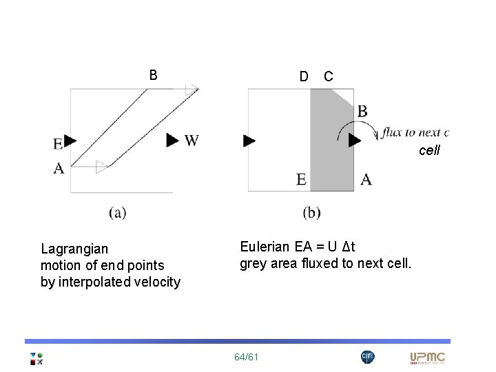
B D C cell Lagrangian motion of end points by interpolated velocity Eulerian EA = U Δt grey area fluxed to next cell. 64/61

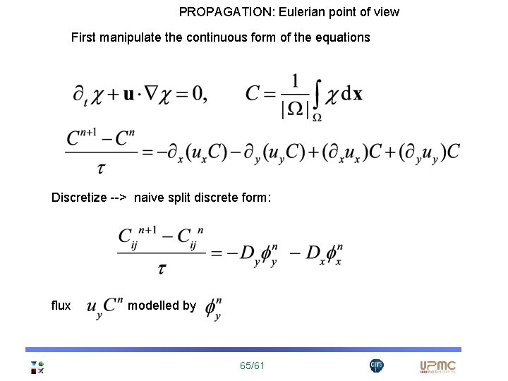
PROPAGATION: Eulerian point of view First manipulate the continuous form of the equations Discretize --> naive split discrete form: flux modelled by 65/61

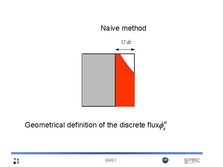
Naive method Geometrical definition of the discrete flux 66/61

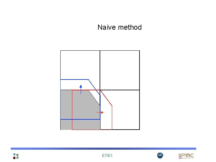
Naive method 67/61

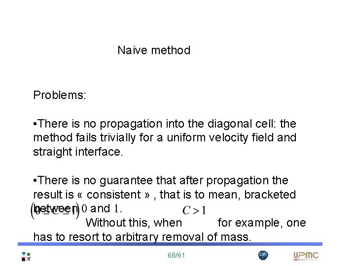
Naive method Problems: • There is no propagation into the diagonal cell: the method fails trivially for a uniform velocity field and straight interface. • There is no guarantee that after propagation the result is « consistent » , that is to mean, bracketed between 0 and 1. Without this, when for example, one has to resort to arbitrary removal of mass. 68/61

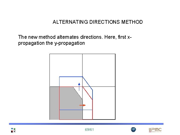
ALTERNATING DIRECTIONS METHOD The new method alternates directions. Here, first xpropagation the y-propagation 69/61

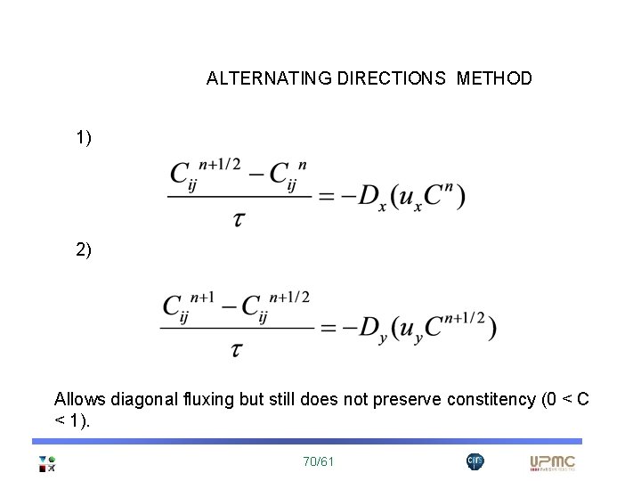
ALTERNATING DIRECTIONS METHOD 1) 2) Allows diagonal fluxing but still does not preserve constitency (0 < C < 1). 70/61

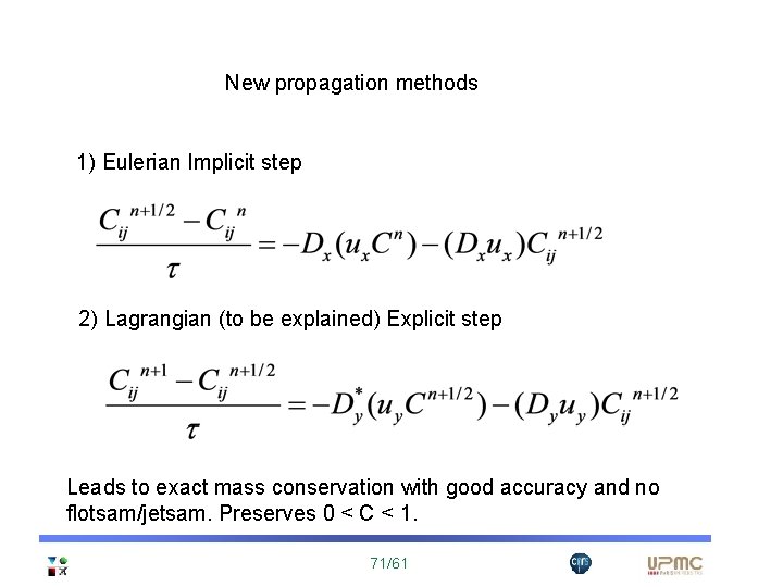
New propagation methods 1) Eulerian Implicit step 2) Lagrangian (to be explained) Explicit step Leads to exact mass conservation with good accuracy and no flotsam/jetsam. Preserves 0 < C < 1. 71/61

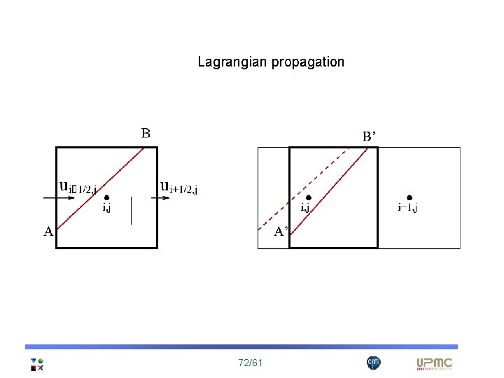
Lagrangian propagation 72/61

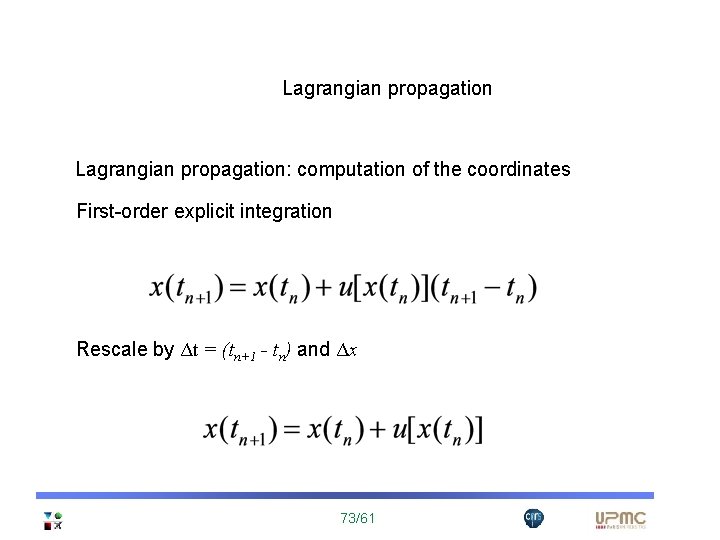
Lagrangian propagation: computation of the coordinates First-order explicit integration Rescale by Δt = (tn+1 - tn) and Δx 73/61

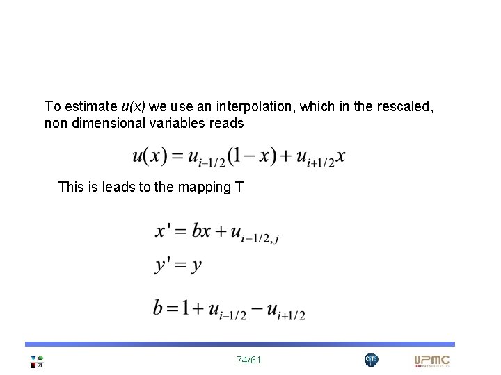
To estimate u(x) we use an interpolation, which in the rescaled, non dimensional variables reads This is leads to the mapping T 74/61

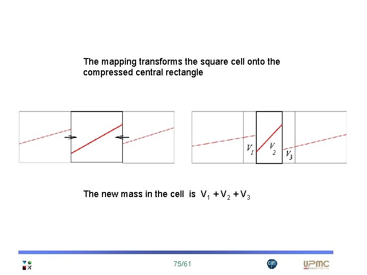
The mapping transforms the square cell onto the compressed central rectangle The new mass in the cell is V 1 + V 2 + V 3 75/61

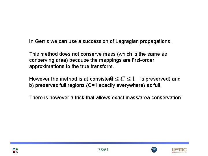
In Gerris we can use a succession of Lagragian propagations. This method does not conserve mass (which is the same as conserving area) because the mappings are first-order approximations to the true transform. However the method is a) consistent is preserved) and b) preserves full regions (C=1 exactly everywhere) as full. There is however a trick that allows exact mass/area conservation 76/61

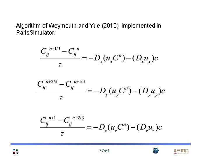
Algorithm of Weymouth and Yue (2010) implemented in Paris. Simulator. 77/61

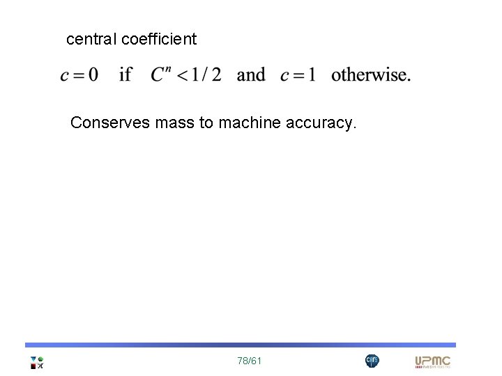
central coefficient Conserves mass to machine accuracy. 78/61