Numerical Descriptive Techniques Measures of Central Location Measures

Numerical Descriptive Techniques Ø Measures of Central Location ü Ø Measures of Variability ü Ø Percentiles, Quartiles Measures of Linear Relationship ü 2 Range, Standard Deviation, Variance, Coefficient of Variation Measures of Relative Standing ü Ø Mean, Median, Mode Covariance, Correlation Jia-Ying Chen

The Arithmetic Mean Ø This is the most popular and useful measure of central location Sum of the observations Mean = Number of observations Ø Drawback ü 3 Very sensitive to extreme values (outliers) Jia-Ying Chen

The Median Ø The Median of a set of observations is the value that falls in the middle when the observations are arranged in order of magnitude. Sample and population medians are computed the same way. Example Comment Suppose only 9 adults were sampled Find the median of the time on the internet (exclude, say, the longest time (33)) for the 10 adults Odd number of observations Even number of observations 0, 0, 5, 5, 7, 7, 8, 8, , 9, 12, 14, 22, 33 0, 330, 5, 7, 8 8 9, 12, 14, 22 8. 5 4 Jia-Ying Chen

The Mode Ø Ø Ø The Mode of a set of observations is the value that occurs most frequently. Set of data may have one mode (or modal class), or two or more modes. When the number of all data appears only once, mode doesn’t exit. The modal class 5 For large data sets the modal class is much more relevant than a single-value mode. Jia-Ying Chen

Example 1 The times (to the nearest minute) that a sample of 9 bank customers waited in line were recorded and are listed here. 7 4 0 2 7 3 1 9 12 Ø Determine the mean, median, and mode for these data. Ø 6 Jia-Ying Chen

Solution 7 Jia-Ying Chen

Relationship among Mean, Median, and Mode Ø If a distribution is symmetrical, the mean, median and mode coincide Ø If a distribution is asymmetrical, and skewed to the left or to the right, the three measures differ. A positively skewed distribution (“skewed to the right”) 8 Mode Mean Median Jia-Ying Chen

Relationship among Mean, Median, and Mode Ø Ø 9 If a distribution is symmetrical, the mean, median and mode coincide If a distribution is non symmetrical, and skewed to the left or to the right, the three measures differ. A positively skewed distribution (“skewed to the right”) A negatively skewed distribution (“skewed to the left”) Mode Mean Median Mean Mode Median Jia-Ying Chen

The range ü ü ü The range of a set of observations is the difference between the largest and smallest observations. Its major advantage is the ease with which it can be computed. Its major shortcoming is its failure to provide information on the dispersion of the observations between the two end points. But, how do all the observations spread out? ? ? ? The range cannot assist. Range in answering this question 10 Smallest observation Largest observation Jia-Ying Chen

Variance… Ø The variance of a population is: population size Ø The variance of a sample is: population mean sample mean Note! the denominator is sample size (n) minus one ! 11 Jia-Ying Chen

Variance… Ø Ø 13 As you can see, you have to calculate the sample mean (x-bar) in order to calculate the sample variance. Alternatively, there is a short-cut formulation to calculate sample variance directly from the data without the intermediate step of calculating the mean. Its given by: Jia-Ying Chen

Proof 14 Jia-Ying Chen

Coefficient of Variation… Ø The coefficient of variation of a set of observations is the standard deviation of the observations divided by their mean, that is: ü ü Ø CV是相對離勢量數（measure of relative disperson） ü ü 15 Population coefficient of variation = CV = Sample coefficient of variation = cv = 1. 比較幾組資料單位不同的差異情形。 2. 比較幾組資料單位相同，但平均數相差懸殊之差異情形。 Jia-Ying Chen

The Empirical Rule… Approximately 68% of all observations fall within one standard deviation of the mean. Approximately 95% of all observations fall within two standard deviations of the mean. Approximately 99. 7% of all observations fall within three standard deviations of the mean. 16 Jia-Ying Chen 4. 16

Chebysheff’s Theorem… A more general interpretation of the standard deviation is derived from Chebysheff’s Theorem, which applies to all shapes of histograms (not just bell shaped). The proportion of observations in any sample that lie within k standard deviations of the mean is at least: For k=2 (say), theorem states that at least 3/4 of all observations lie within 2 standard deviations of the mean. This is a “lower bound” compared to Empirical Rule’s approximation (95%). 17 Jia-Ying Chen 4. 17

Example 2 Ø Determine the variance, standard deviation, range, and the cv of the following sample. 9 15 11 31 23 13 15 17 21 18 Jia-Ying Chen

Solution 19 Jia-Ying Chen

Measures of Relative Standing and Box Plots Ø Percentile ü The pth percentile of a set of measurements is the value for which p percent of the observations are less than that value l 100(1 -p) percent of all the observations are greater than that value. l ü Example l Suppose your score is the 60% percentile of a SAT test. Then 60% of all the scores lie here 21 Your score 40% Jia-Ying Chen

Quartiles Ø Commonly used percentiles ü ü ü 22 First (lower)decile First (lower) quartile, Q 1, Second (middle)quartile, Q 2, Third quartile, Q 3, Ninth (upper)decile = 10 th percentile = 25 th percentile = 50 th percentile = 75 th percentile = 90 th percentile Jia-Ying Chen

Location of Percentiles Ø 23 Find the location of any percentile using the formula Jia-Ying Chen

Example 4 Ø Determine the first, second, and third quartiles of the following data 10. 5 14. 7 15. 3 17. 7 15. 9 12. 2 10. 0 14. 1 13. 9 18. 5 13. 9 15. 1 14. 7 24 Jia-Ying Chen

Solution Ø 排序後數列 ü Ø Ø Ø 25 10. 0 10. 5 12. 2 13. 9 14. 1 14. 7 15. 1 15. 3 15. 9 17. 7 18. 5 First quartile: L 25=(13+1)*25/100=3. 5; the first quartile is 13. 05 Second quartile: L 50=(13+1)*50/100=7; the first quartile is 14. 7 Third quartile: L 75=(13+1)*75/100=10. 5; the first quartile is 15. 6 Jia-Ying Chen

Interquartile Range Ø Ø This is a measure of the spread of the middle 50% of the observations Large value indicates a large spread of the observations Interquartile range = Q 3 – Q 1 26 Jia-Ying Chen

Box Plot ü This is a pictorial display that provides the main descriptive measures of the data set: l l l L - the largest observation Q 3 - The upper quartile Q 2 - The median Q 1 - The lower quartile S - The smallest observation 1. 5(Q 3 – Q 1) Whisker S Q 1 27 1. 5(Q 3 – Q 1) Q 2 Q 3 Whisker L Jia-Ying Chen

Measures of Linear Relationship… Ø Ø 28 We now present two numerical measures of linear relationship that provide information as to the strength & direction of a linear relationship between two variables (if one exists). They are the covariance and the coefficient of correlation. Covariance - is there any pattern to the way two variables move together? Coefficient of correlation - how strong is the linear relationship between two variables? Jia-Ying Chen

Covariance… population mean of variable X, variable Y sample mean of variable X, variable Y Note: divisor is n-1, not n as you may expect. 29 Jia-Ying Chen

Covariance… Ø 30 In much the same way there was a “shortcut” for calculating sample variance without having to calculate the sample mean, there is also a shortcut for calculating sample covariance without having to first calculate the mean: Jia-Ying Chen

Covariance… (Generally speaking) ØWhen two variables move in the same direction (both increase or both decrease), the covariance will be a large positive number. ØWhen two variables move in opposite directions, the covariance is a large negative number. ØWhen there is no particular pattern, the covariance is a small number. 31 Jia-Ying Chen

Coefficient of Correlation… Ø The coefficient of correlation is defined as the covariance divided by the standard deviations of the variables: Greek letter “rho” This coefficient answers the question: How strong is the association between X and Y? 32 Jia-Ying Chen

Coefficient of Correlation… ØThe advantage of the coefficient of correlation over covariance is that it has fixed range from -1 to +1, thus: ØIf the two variables are very strongly positively related, the coefficient value is close to +1 (strong positive linear relationship). ØIf the two variables are very strongly negatively related, the coefficient value is close to -1 (strong negative linear relationship). ØNo straight line relationship is indicated by a coefficient close to zero. 33 Jia-Ying Chen

Coefficient of Correlation… +1 Strong positive linear relationship r or r = 0 No linear relationship -1 Strong negative linear relationship 34 Jia-Ying Chen

Example 5 Are the marks one receives in a course related to the amount of time spent studying the subject? To analyze this mysterious possibility, a student took a random sample of 10 students who had enrolled in an accounting class last semester. She asked each to report his or her mark in the course and the total number of hours spent studying accounting. These data are listed here. Time Spent Studying 40 42 37 47 25 44 41 48 35 28 Marks 77 63 79 86 51 78 83 90 65 47 Ø a. Calculate the covariance Ø b. Calculate the coefficient of correlation Ø c. What do the statistics calculated above tell you about the relationship between marks and study time? Ø 35 Jia-Ying Chen

Solution 36 Jia-Ying Chen

Solution 37 Jia-Ying Chen

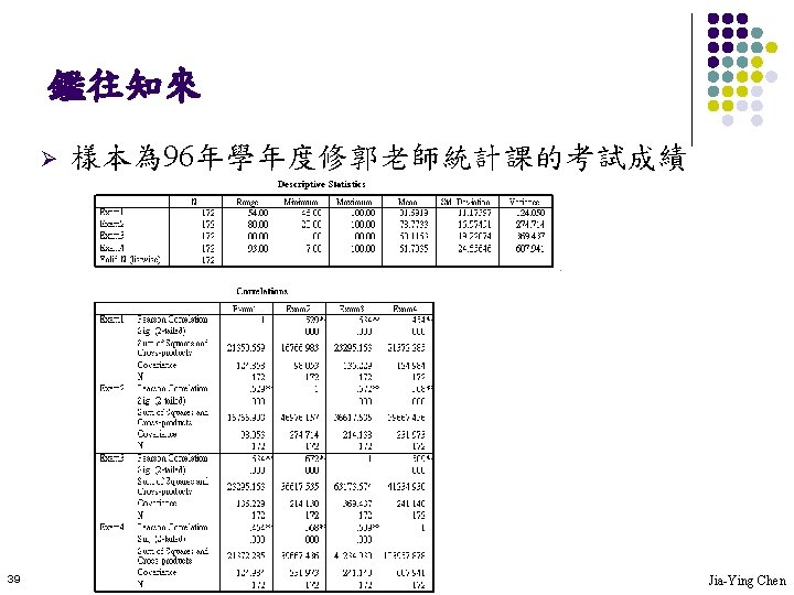
Solution Ø 38 c. There is a strong positive linear relationship between marks and study time. Jia-Ying Chen