Spline Interpolation Method Civil Engineering Majors Authors Autar

Spline Interpolation Method Civil Engineering Majors Authors: Autar Kaw, Jai Paul http: //numericalmethods. eng. usf. edu Transforming Numerical Methods Education for STEM Undergraduates http: //numericalmethods. eng. usf. edu 1

Spline Method of Interpolation http: //numericalmethods. eng. usf. edu

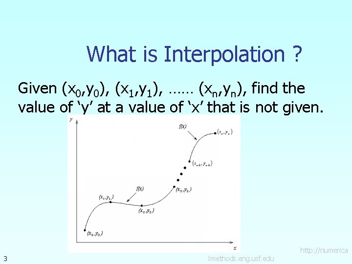
What is Interpolation ? Given (x 0, y 0), (x 1, y 1), …… (xn, yn), find the value of ‘y’ at a value of ‘x’ that is not given. 3 lmethods. eng. usf. edu http: //numerica

Interpolants Polynomials are the most common choice of interpolants because they are easy to: Evaluate Differentiate, and Integrate. 4 lmethods. eng. usf. edu http: //numerica

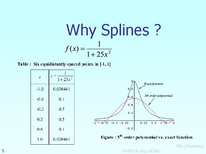
Why Splines ? 5 lmethods. eng. usf. edu http: //numerica

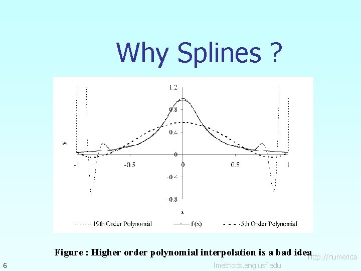
Why Splines ? 6 Figure : Higher order polynomial interpolation is a bad ideahttp: //numerica lmethods. eng. usf. edu

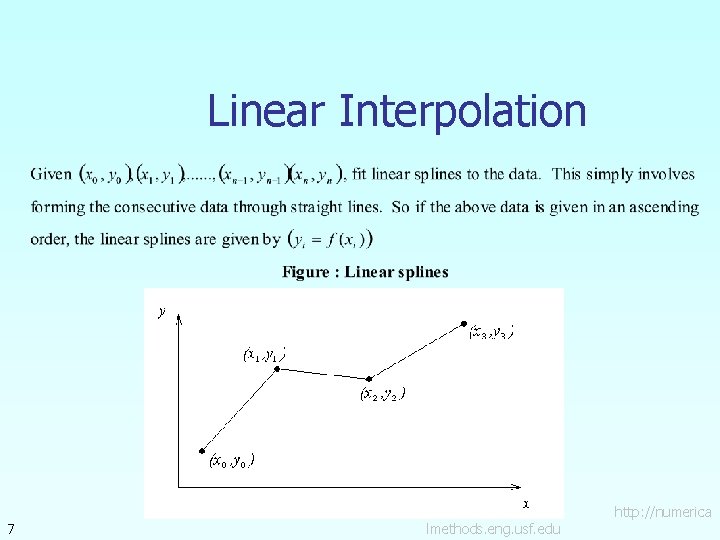
Linear Interpolation 7 lmethods. eng. usf. edu http: //numerica

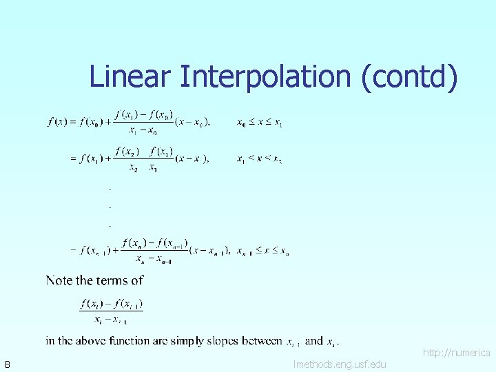
Linear Interpolation (contd) 8 lmethods. eng. usf. edu http: //numerica

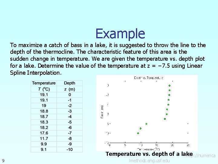
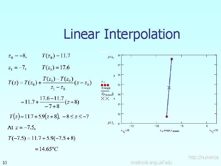
Example To maximize a catch of bass in a lake, it is suggested to throw the line to the depth of thermocline. The characteristic feature of this area is the sudden change in temperature. We are given the temperature vs. depth plot for a lake. Determine the value of the temperature at z = − 7. 5 using Linear Spline Interpolation. 9 Temperature vs. depth of a lake http: //numerica lmethods. eng. usf. edu

Linear Interpolation 10 lmethods. eng. usf. edu http: //numerica

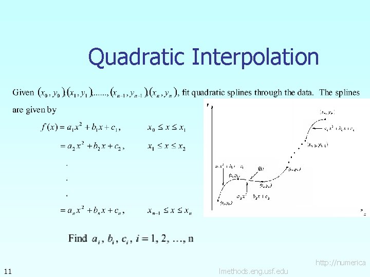
Quadratic Interpolation 11 lmethods. eng. usf. edu http: //numerica

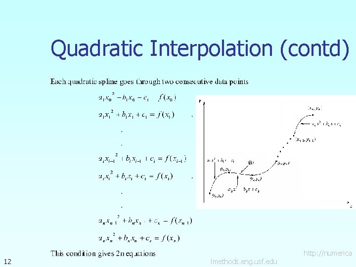
Quadratic Interpolation (contd) 12 lmethods. eng. usf. edu http: //numerica

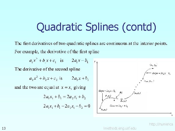
Quadratic Splines (contd) 13 lmethods. eng. usf. edu http: //numerica

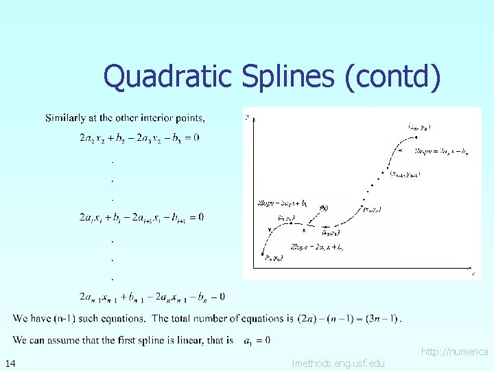
Quadratic Splines (contd) 14 lmethods. eng. usf. edu http: //numerica

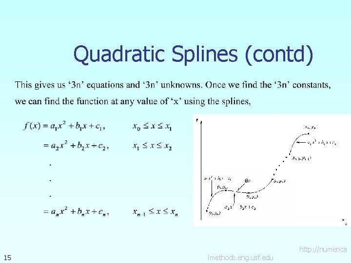
Quadratic Splines (contd) 15 lmethods. eng. usf. edu http: //numerica

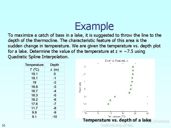
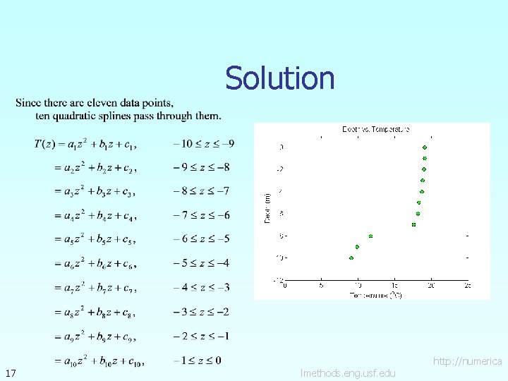
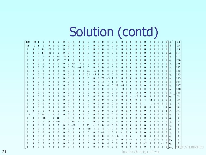
Example To maximize a catch of bass in a lake, it is suggested to throw the line to the depth of thermocline. The characteristic feature of this area is the sudden change in temperature. We are given the temperature vs. depth plot for a lake. Determine the value of the temperature at z = − 7. 5 using Quadratic Spline Interpolation. 16 Temperature vs. depth of a lake http: //numerica lmethods. eng. usf. edu

Solution 17 lmethods. eng. usf. edu http: //numerica

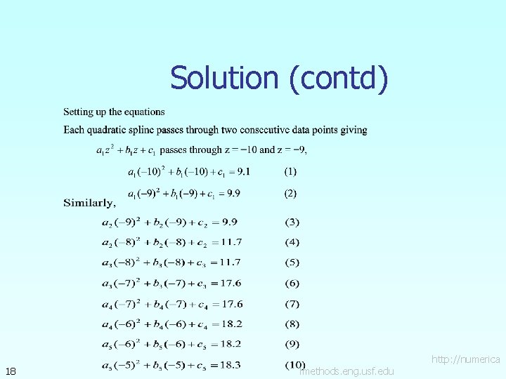
Solution (contd) 18 lmethods. eng. usf. edu http: //numerica

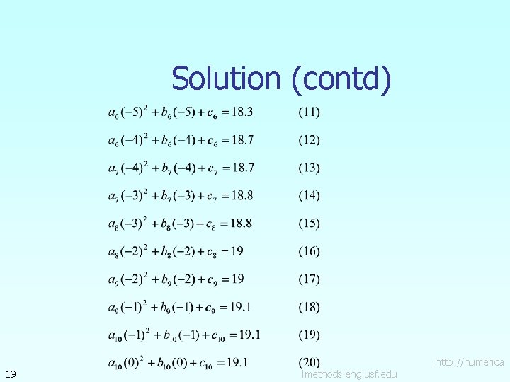
Solution (contd) 19 lmethods. eng. usf. edu http: //numerica

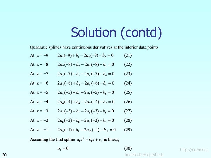
Solution (contd) 20 lmethods. eng. usf. edu http: //numerica

Solution (contd) 21 lmethods. eng. usf. edu http: //numerica

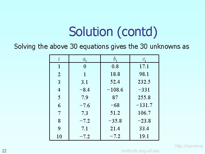
Solution (contd) Solving the above 30 equations gives the 30 unknowns as i 1 2 3 4 5 6 7 8 9 10 22 ai 0 1 3. 1 − 8. 4 7. 9 − 7. 6 7. 3 − 7. 2 7. 1 − 7. 2 bi 0. 8 18. 8 52. 4 − 108. 6 87 − 68 51. 2 − 35. 8 21. 4 − 7. 2 ci 17. 1 98. 1 232. 5 − 331 255. 8 − 131. 7 106. 7 − 23. 8 33. 4 19. 1 lmethods. eng. usf. edu http: //numerica

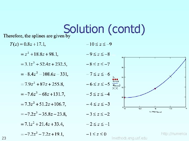
Solution (contd) 23 lmethods. eng. usf. edu http: //numerica

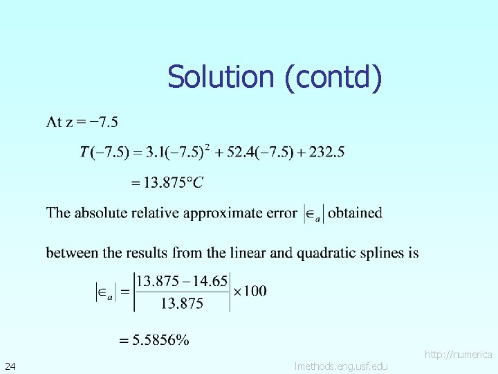
Solution (contd) 24 lmethods. eng. usf. edu http: //numerica

Additional Resources For all resources on this topic such as digital audiovisual lectures, primers, textbook chapters, multiple-choice tests, worksheets in MATLAB, MATHEMATICA, Math. Cad and MAPLE, blogs, related physical problems, please visit http: //numericalmethods. eng. usf. edu/topics/spline_me thod. html

THE END http: //numericalmethods. eng. usf. edu