Advanced Computer Programming Search Algorithms Sinan AYDIN Search


- Slides: 13

Advanced Computer Programming Search Algorithms Sinan AYDIN

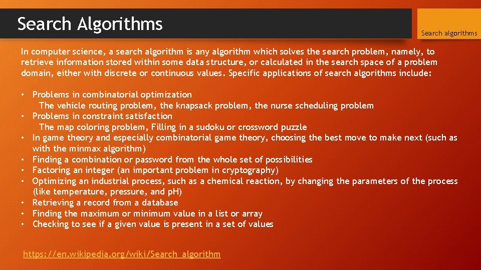
Search Algorithms Search algorithms In computer science, a search algorithm is any algorithm which solves the search problem, namely, to retrieve information stored within some data structure, or calculated in the search space of a problem domain, either with discrete or continuous values. Specific applications of search algorithms include: • Problems in combinatorial optimization The vehicle routing problem, the knapsack problem, the nurse scheduling problem • Problems in constraint satisfaction The map coloring problem, Filling in a sudoku or crossword puzzle • In game theory and especially combinatorial game theory, choosing the best move to make next (such as with the minmax algorithm) • Finding a combination or password from the whole set of possibilities • Factoring an integer (an important problem in cryptography) • Optimizing an industrial process, such as a chemical reaction, by changing the parameters of the process (like temperature, pressure, and p. H) • Retrieving a record from a database • Finding the maximum or minimum value in a list or array • Checking to see if a given value is present in a set of values https: //en. wikipedia. org/wiki/Search_algorithm

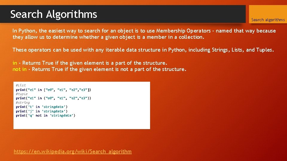
Search Algorithms Search algorithms In Python, the easiest way to search for an object is to use Membership Operators - named that way because they allow us to determine whether a given object is a member in a collection. These operators can be used with any iterable data structure in Python, including Strings, Lists, and Tuples. in - Returns True if the given element is a part of the structure. not in - Returns True if the given element is not a part of the structure. #List print("e 1" in ["e 0", "e 1", "e 2", "e 3"]) #tuple print("e 1" in ("e 0", "e 1", "e 2", "e 3")) #string print('t' in 'stringdata') print('j' in 'stringdata') print('q' not in 'stringdata') https: //en. wikipedia. org/wiki/Search_algorithm

Search algorithms Searching Algorithms : 1. Linear Search 2. Binary Search 3. Jump Search 4. Interpolation Search 5. Exponential Search 6. Sublist Search (Search a linked list in another list) 7. Fibonacci Search 8. The Ubiquitous Binary Search 9. Recursive program to linearly search an element in a given array 10. Recursive function to do substring search 11. Unbounded Binary Search algorithms

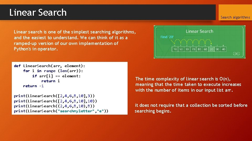
Linear Search algorithms Linear search is one of the simplest searching algorithms, and the easiest to understand. We can think of it as a ramped-up version of our own implementation of Python's in operator. def Linear. Search(arr, element): for i in range (len(arr)): if arr[i] == element: return i return -1 print(Linear. Search([2, 4, 6, 8, 10], 3)) print(Linear. Search([2, 4, 6, 8, 10], 10)) print(Linear. Search((2, 4, 6, 8, 10), 8)) print(Linear. Search("searchmyletter", "e")) The time complexity of linear search is O(n), meaning that the time taken to execute increases with the number of items in our input list arr. it does not require that a collection be sorted before searching begins.

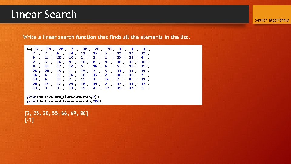
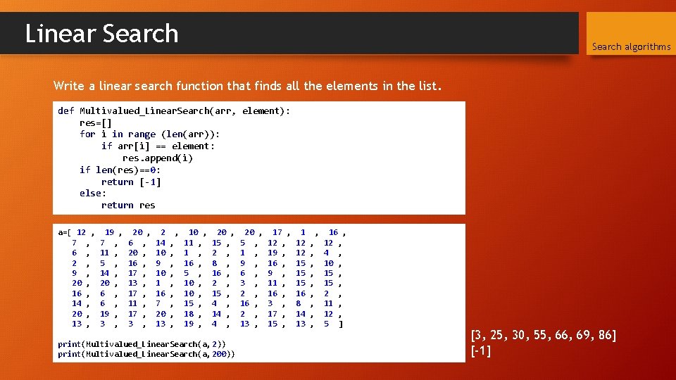
Linear Search algorithms Write a linear search function that finds all the elements in the list. a=[ 12 , 7 , 6 , 2 , 9 , 20 , 16 , 14 , 20 , 13 , 19 , 7 , 11 , 5 , 14 , 20 , 6 , 19 , 3 , 20 , 6 , 20 , 16 , 17 , 13 , 17 , 11 , 17 , 3 , 2 14 10 9 10 1 16 7 20 13 , , , , , 10 , 11 , 16 , 5 , 10 , 15 , 18 , 19 , 20 , 15 , 2 , 8 , 16 , 2 , 15 , 4 , 14 , print(Multivalued_Linear. Search(a, 2)) print(Multivalued_Linear. Search(a, 200)) [3, 25, 30, 55, 66, 69, 86] [-1] 20 , 5 , 1 , 9 , 6 , 3 , 2 , 16 , 2 , 13 , 17 , 12 , 19 , 16 , 9 , 11 , 16 , 3 , 17 , 15 , 1 12 12 15 15 15 16 8 14 13 , , , , , 16 , 12 , 4 , 10 , 15 , 2 , 11 , 12 , 5 ]

Linear Search algorithms Write a linear search function that finds all the elements in the list. def Multivalued_Linear. Search(arr, element): res=[] for i in range (len(arr)): if arr[i] == element: res. append(i) if len(res)==0: return [-1] else: return res a=[ 12 , 7 , 6 , 2 , 9 , 20 , 16 , 14 , 20 , 13 , 19 , 7 , 11 , 5 , 14 , 20 , 6 , 19 , 3 , 20 , 6 , 20 , 16 , 17 , 13 , 17 , 11 , 17 , 3 , 2 14 10 9 10 1 16 7 20 13 , , , , , 10 , 11 , 16 , 5 , 10 , 15 , 18 , 19 , 20 , 15 , 2 , 8 , 16 , 2 , 15 , 4 , 14 , print(Multivalued_Linear. Search(a, 2)) print(Multivalued_Linear. Search(a, 200)) 20 , 5 , 1 , 9 , 6 , 3 , 2 , 16 , 2 , 13 , 17 , 12 , 19 , 16 , 9 , 11 , 16 , 3 , 17 , 15 , 1 12 12 15 15 15 16 8 14 13 , , , , , 16 , 12 , 4 , 10 , 15 , 2 , 11 , 12 , 5 ] [3, 25, 30, 55, 66, 69, 86] [-1]

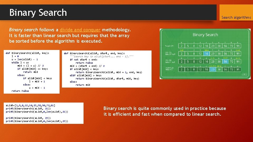
Binary Search algorithms Binary search follows a divide and conquer methodology. It is faster than linear search but requires that the array be sorted before the algorithm is executed. def Binary. Search 1(alist, key): l = 0 u = len(alist) - 1 while l < u: mid = (l + u) // 2 if alist[mid] == key: return mid else: if alist[mid] < key: l = mid + 1 else: u = mid - 1 return False def Binary. Search 2(alist, start, end, key): """Search key in alist[start. . . end - 1]. """ if not start < end: return False mid = (start + end) // 2 if alist[mid] < key: return Binary. Search 2(alist, mid + 1, end, key) elif alist[mid] > key: return Binary. Search 2(alist, start, mid, key) else: return mid a. List=[1, 5, 8, 12, 16, 23, 38, 56, 72, 91] print(Binary. Search 1(a. List, 21)) print(Binary. Search 2(a. List, 0, len(a. List), 21)) print(Binary. Search 1(a. List, 23)) print(Binary. Search 2(a. List, 0, len(a. List), 23)) Binary search is quite commonly used in practice because it is efficient and fast when compared to linear search.

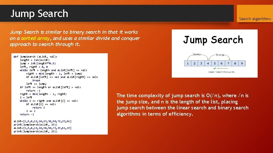
Jump Search algorithms Jump Search is similar to binary search in that it works on a sorted array, and uses a similar divide and conquer approach to search through it. def Jump. Search (a. List, val): length = len(a. List) jump = int(length**0. 5) left, right = 0, 0 while left < length and a. List[left] <= val: right = min(length - 1, left + jump) if a. List[left] <= val and a. List[right] >= val: break left += jump; if left >= length or a. List[left] > val: return -1 right = min(length - 1, right) i = left while i <= right and a. List[i] <= val: if a. List[i] == val: return i i += 1 return -1 a. List=[1, 5, 8, 12, 16, 23, 38, 56, 72, 23, 91] print(Jump. Search(a. List, 23)) a. List=[1, 5, 8, 12, 16, 38, 56, 72, 23, 91, 23] print(Jump. Search(a. List, 23)) The time complexity of jump search is O(√n), where √n is the jump size, and n is the length of the list, placing jump search between the linear search and binary search algorithms in terms of efficiency.

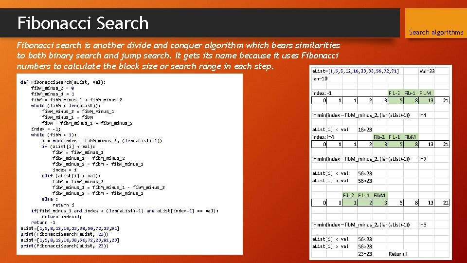
Fibonacci Search Fibonacci search is another divide and conquer algorithm which bears similarities to both binary search and jump search. It gets its name because it uses Fibonacci numbers to calculate the block size or search range in each step. def Fibonacci. Search(a. List, val): fib. M_minus_2 = 0 fib. M_minus_1 = 1 fib. M = fib. M_minus_1 + fib. M_minus_2 while (fib. M < len(a. List)): fib. M_minus_2 = fib. M_minus_1 = fib. M_minus_1 + fib. M_minus_2 index = -1; while (fib. M > 1): i = min(index + fib. M_minus_2, (len(a. List)-1)) if (a. List[i] < val): fib. M = fib. M_minus_1 = fib. M_minus_2 = fib. M - fib. M_minus_1 index = i elif (a. List[i] > val): fib. M = fib. M_minus_2 fib. M_minus_1 = fib. M_minus_1 - fib. M_minus_2 = fib. M - fib. M_minus_1 else : return i if(fib. M_minus_1 and index < (len(a. List)-1) and a. List[index+1] == val): return index+1; return -1 a. List=[1, 5, 8, 12, 16, 23, 38, 56, 72, 23, 91] print(Fibonacci. Search(a. List, 23)) a. List=[1, 5, 8, 12, 16, 38, 56, 72, 23, 91, 23] print(Fibonacci. Search(a. List, 23)) Search algorithms

Fibonacci Search algorithms The time complexity for Fibonacci search is O(log n); the same as binary search. This means the algorithm is faster than both linear search and jump search in most cases. Fibonacci search can be used when we have a very large number of elements to search through, and we want to reduce the inefficiency associated with using an algorithm which relies on the division operator. An additional advantage of using Fibonacci search is that it can accommodate input arrays that are too large to be held in CPU cache or RAM, because it searches through elements in increasing step sizes, and not in a fixed size.

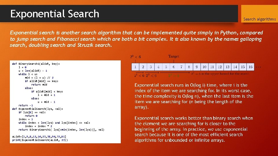
Exponential Search algorithms Exponential search is another search algorithm that can be implemented quite simply in Python, compared to jump search and Fibonacci search which are both a bit complex. It is also known by the names galloping search, doubling search and Struzik search. def Binary. Search 1(alist, key): l = 0 u = len(alist) - 1 while l < u: mid = (l + u) // 2 if alist[mid] == key: return mid else: if alist[mid] < key: l = mid + 1 else: u = mid - 1 return -1 def Exponential. Search(lys, val): if lys[0] == val: return 0 index = 1 while index < len(lys) and lys[index] <= val: index = index * 2 return Binary. Search 1( lys[: min(index, len(lys))], val) a. List=[1, 5, 8, 12, 16, 23, 38, 56, 72, 91] print(Exponential. Search(a. List, 23))

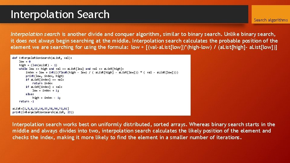
Interpolation Search algorithms Interpolation search is another divide and conquer algorithm, similar to binary search. Unlike binary search, it does not always begin searching at the middle. Interpolation search calculates the probable position of the element we are searching for using the formula: low + [(val-a. List[low])*(high-low) / (a. List[high]- a. List[low])] def Interpolation. Search(a. List, val): low = 0 high = (len(a. List) - 1) while low <= high and val >= a. List[low] and val <= a. List[high]: index = low + int(((float(high - low) / ( a. List[high] - a. List[low])) * ( val - a. List[low]))) print(low, index, high) if a. List[index] == val: return index if a. List[index] < val: low = index + 1; else: high = index - 1; return -1 a. List=[1, 5, 8, 12, 16, 23, 38, 56, 72, 91] print(Interpolation. Search(a. List, 23)) Interpolation search works best on uniformly distributed, sorted arrays. Whereas binary search starts in the middle and always divides into two, interpolation search calculates the likely position of the element and checks the index, making it more likely to find the element in a smaller number of iterations.