Engineering Computation Curve Fitting Interpolation 1 Curve Fitting

Engineering Computation Curve Fitting: Interpolation 1 Curve Fitting by Interpolation

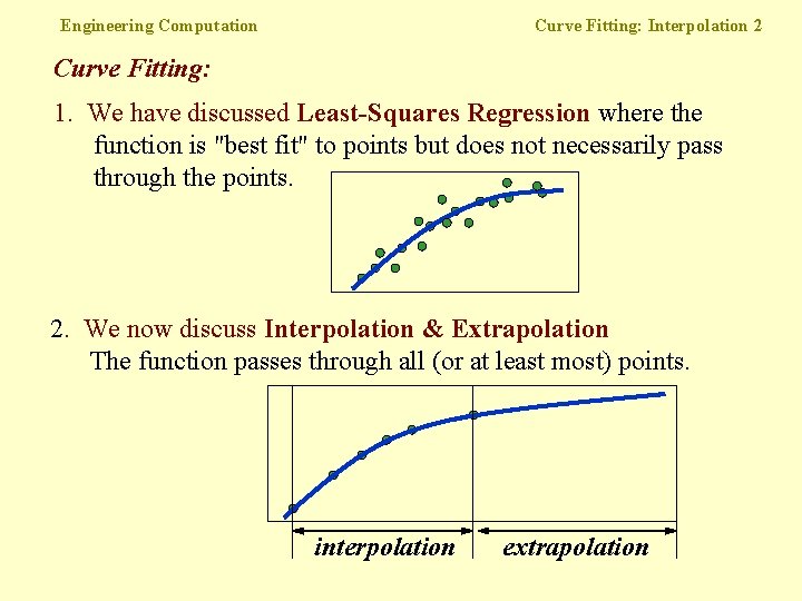
Engineering Computation Curve Fitting: Interpolation 2 Curve Fitting: 1. We have discussed Least-Squares Regression where the function is "best fit" to points but does not necessarily pass through the points. 2. We now discuss Interpolation & Extrapolation The function passes through all (or at least most) points. interpolation extrapolation

Engineering Computation Curve Fitting: Interpolation 3 Curve Fitting by Interpolation: C&C covers four approaches: 1. Polynomials (C&C 18. 1 -18. 5 – “skim” only) a) n + 1 equations & n + 1 unknowns b) Lagrange Polynomials c) Newton's Divided Difference (NDD) Polynomials 2. Splines (C&C 18. 6 – assigned reading) The first 3 approaches find the same polynomial. We will only cover superficially, and concentrate on Splines.

Engineering Computation Curve Fitting: Interpolation 4 Curve Fitting by Interpolation: General Scheme Given: Set of points (xi, yi), not necessarily evenly spaced or in ascending order. Assume: x = independent variable; y = dependent variable. Find: y = f(x) at some value of x not in the set (xi). Method: Determine the function f(x) which passes through all (or most) points.

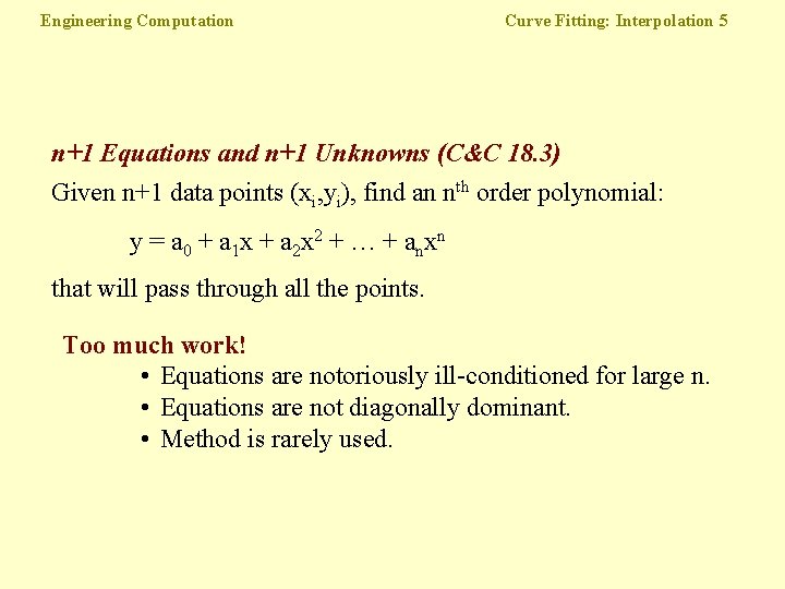
Engineering Computation Curve Fitting: Interpolation 5 n+1 Equations and n+1 Unknowns (C&C 18. 3) Given n+1 data points (xi, yi), find an nth order polynomial: y = a 0 + a 1 x + a 2 x 2 + … + anxn that will pass through all the points. Too much work! • Equations are notoriously ill-conditioned for large n. • Equations are not diagonally dominant. • Method is rarely used.

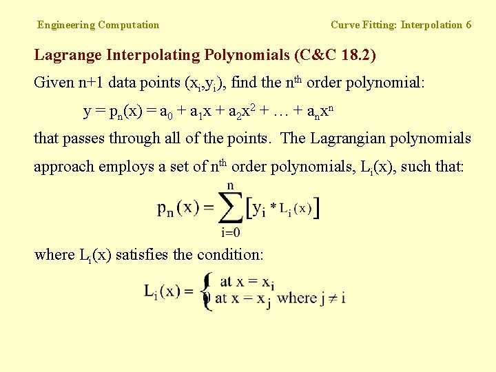
Engineering Computation Curve Fitting: Interpolation 6 Lagrange Interpolating Polynomials (C&C 18. 2) Given n+1 data points (xi, yi), find the nth order polynomial: y = pn(x) = a 0 + a 1 x + a 2 x 2 + … + anxn that passes through all of the points. The Lagrangian polynomials approach employs a set of nth order polynomials, Li(x), such that: where Li(x) satisfies the condition:

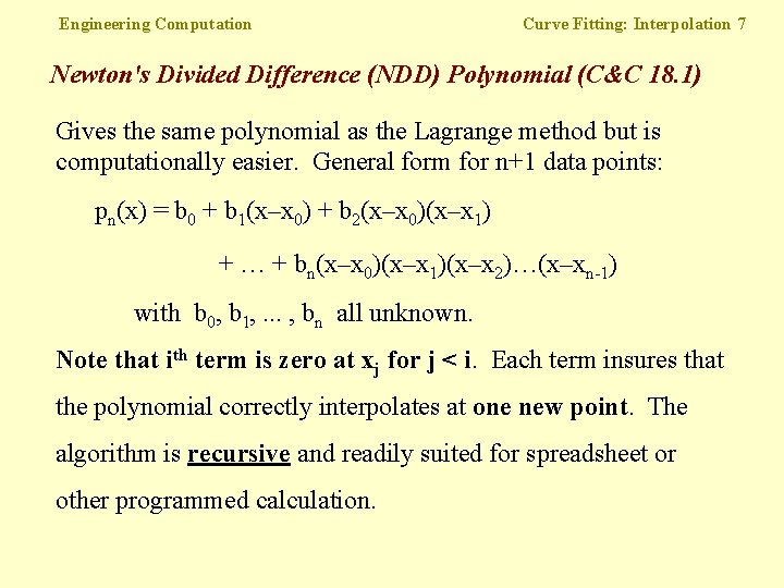
Engineering Computation Curve Fitting: Interpolation 7 Newton's Divided Difference (NDD) Polynomial (C&C 18. 1) Gives the same polynomial as the Lagrange method but is computationally easier. General form for n+1 data points: pn(x) = b 0 + b 1(x–x 0) + b 2(x–x 0)(x–x 1) + … + bn(x–x 0)(x–x 1)(x–x 2)…(x–xn-1) with b 0, b 1, . . . , bn all unknown. Note that ith term is zero at xj for j < i. Each term insures that the polynomial correctly interpolates at one new point. The algorithm is recursive and readily suited for spreadsheet or other programmed calculation.

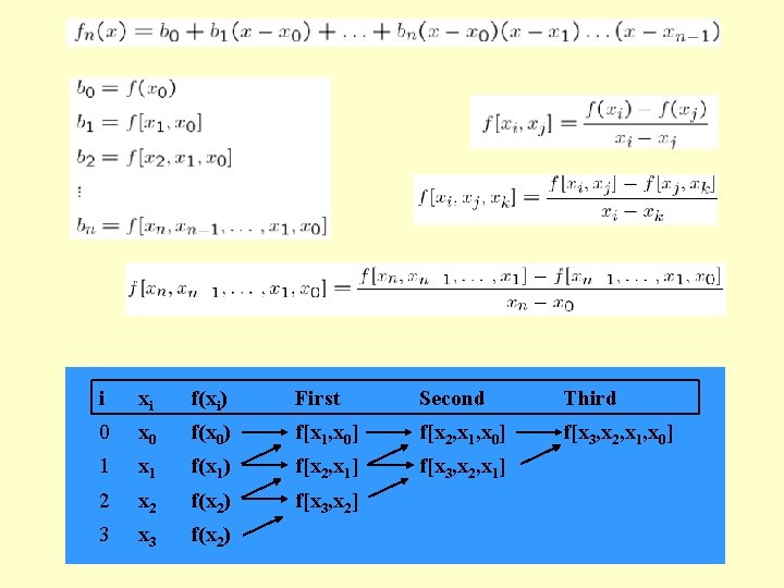
i xi f(xi) First Second Third 0 x 0 f(x 0) f[x 1, x 0] f[x 2, x 1, x 0] f[x 3, x 2, x 1, x 0] 1 x 1 f(x 1) f[x 2, x 1] f[x 3, x 2, x 1] 2 x 2 f(x 2) f[x 3, x 2] 3 x 3 f(x 2)

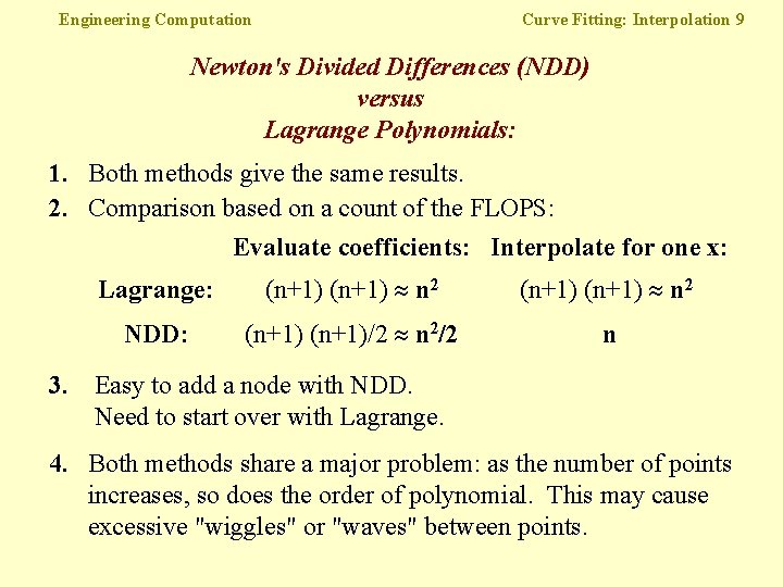
Engineering Computation Curve Fitting: Interpolation 9 Newton's Divided Differences (NDD) versus Lagrange Polynomials: 1. Both methods give the same results. 2. Comparison based on a count of the FLOPS: Evaluate coefficients: Interpolate for one x: Lagrange: (n+1) n 2 NDD: (n+1)/2 n 2/2 n 3. Easy to add a node with NDD. Need to start over with Lagrange. 4. Both methods share a major problem: as the number of points increases, so does the order of polynomial. This may cause excessive "wiggles" or "waves" between points.

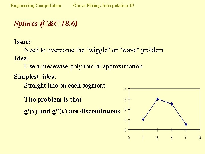
Engineering Computation Curve Fitting: Interpolation 10 Splines (C&C 18. 6) Issue: Need to overcome the "wiggle" or "wave" problem Idea: Use a piecewise polynomial approximation Simplest idea: Straight line on each segment. The problem is that g'(x) and g"(x) are discontinuous

Engineering Computation Curve Fitting: Interpolation 11 Splines (cont. ) Most frequently used: Cubic Splines ==> Separate Cubic polynomial on each interval. This is the analytical/numerical analog of a flexible edge (spline) which is used by draftsmen. With this tool the first and second derivatives (curvature) are continuous, and the function appears "smooth".

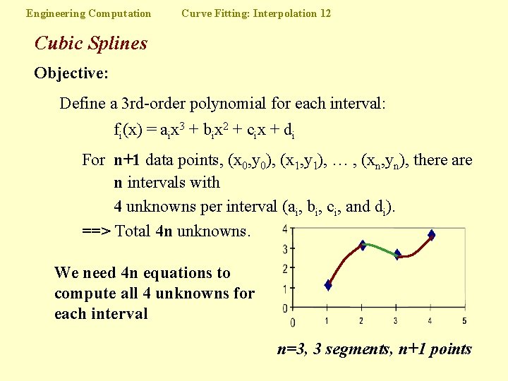
Engineering Computation Curve Fitting: Interpolation 12 Cubic Splines Objective: Define a 3 rd-order polynomial for each interval: fi(x) = aix 3 + bix 2 + cix + di For n+1 data points, (x 0, y 0), (x 1, y 1), … , (xn, yn), there are n intervals with 4 unknowns per interval (ai, bi, ci, and di). ==> Total 4 n unknowns. We need 4 n equations to compute all 4 unknowns for each interval n=3, 3 segments, n+1 points

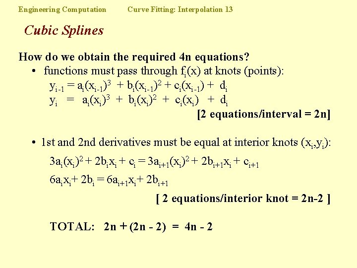
Engineering Computation Curve Fitting: Interpolation 13 Cubic Splines How do we obtain the required 4 n equations? • functions must pass through fi(x) at knots (points): yi-1 = ai(xi-1)3 + bi(xi-1)2 + ci(xi-1) + di yi = ai(xi)3 + bi(xi)2 + ci(xi) + di [2 equations/interval = 2 n] • 1 st and 2 nd derivatives must be equal at interior knots (xi, yi): 3 ai(xi)2 + 2 bixi + ci = 3 ai+1(xi)2 + 2 bi+1 xi + ci+1 6 aixi+ 2 bi = 6 ai+1 xi+ 2 bi+1 [ 2 equations/interior knot = 2 n-2 ] TOTAL: 2 n + (2 n - 2) = 4 n - 2

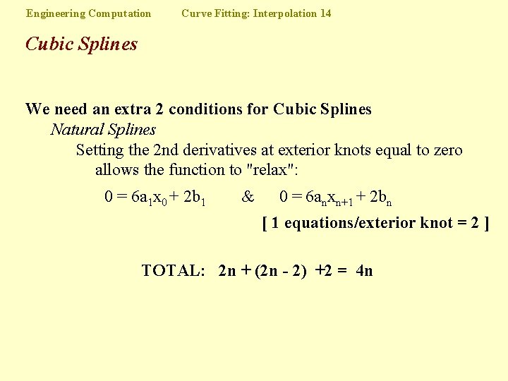
Engineering Computation Curve Fitting: Interpolation 14 Cubic Splines We need an extra 2 conditions for Cubic Splines Natural Splines Setting the 2 nd derivatives at exterior knots equal to zero allows the function to "relax": 0 = 6 a 1 x 0 + 2 b 1 & 0 = 6 anxn+1 + 2 bn [ 1 equations/exterior knot = 2 ] TOTAL: 2 n + (2 n - 2) +2 = 4 n

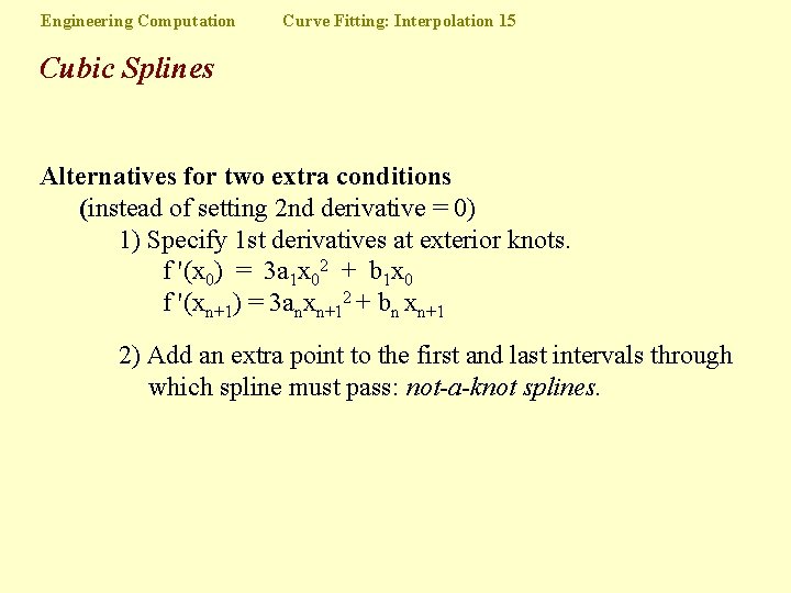
Engineering Computation Curve Fitting: Interpolation 15 Cubic Splines Alternatives for two extra conditions (instead of setting 2 nd derivative = 0) 1) Specify 1 st derivatives at exterior knots. f '(x 0) = 3 a 1 x 02 + b 1 x 0 f '(xn+1) = 3 anxn+12 + bn xn+1 2) Add an extra point to the first and last intervals through which spline must pass: not-a-knot splines.

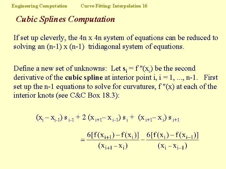
Engineering Computation Curve Fitting: Interpolation 16 Cubic Splines Computation If set up cleverly, the 4 n x 4 n system of equations can be reduced to solving an (n-1) x (n-1) tridiagonal system of equations. Define a new set of unknowns: Let si = f "(xi) be the second derivative of the cubic spline at interior point i, i = 1, . . . , n-1. First set up the n-1 equations to solve for curvatures, f "(x) at each of the interior knots (see C&C Box 18. 3): (xi – xi-1) s i-1 + 2 (x i+1– x i-1) s i + (x i+1– x i) s i+1

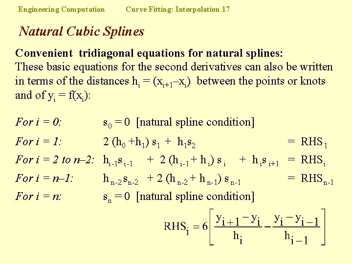
Engineering Computation Curve Fitting: Interpolation 17 Natural Cubic Splines Convenient tridiagonal equations for natural splines: These basic equations for the second derivatives can also be written in terms of the distances hi = (xi+1–xi) between the points or knots and of yi = f(xi): For i = 0: s 0 = 0 [natural spline condition] For i = 1: 2 (h 0 +h 1) s 1 + h 1 s 2 For i = 2 to n– 2: hi-1 s i-1 + 2 (h i-1 + h i) s i = RHS 1 + h is i+1 = RHSi For i = n– 1: h n-2 sn-2 + 2 (h n-2 + h n-1) s n-1 For i = n: sn = 0 [natural spline condition] = RHSn-1

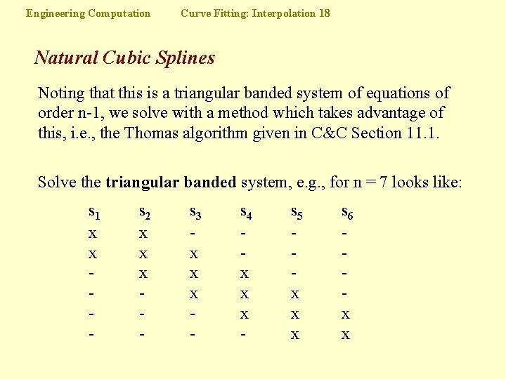
Engineering Computation Curve Fitting: Interpolation 18 Natural Cubic Splines Noting that this is a triangular banded system of equations of order n-1, we solve with a method which takes advantage of this, i. e. , the Thomas algorithm given in C&C Section 11. 1. Solve the triangular banded system, e. g. , for n = 7 looks like: s 1 x x - s 2 x x x - s 3 x x x - s 4 x x x - s 5 x x x s 6 x x

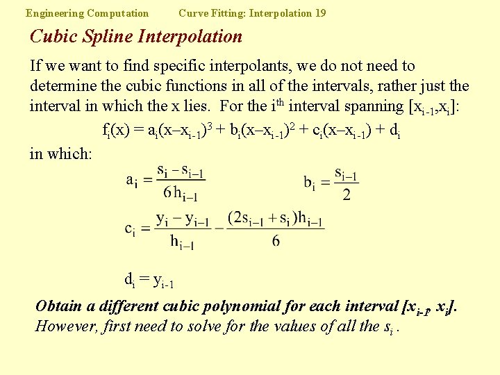
Engineering Computation Curve Fitting: Interpolation 19 Cubic Spline Interpolation If we want to find specific interpolants, we do not need to determine the cubic functions in all of the intervals, rather just the interval in which the x lies. For the ith interval spanning [xi-1, xi]: fi(x) = ai(x–xi-1)3 + bi(x–xi-1)2 + ci(x–xi-1) + di in which: di = yi-1 Obtain a different cubic polynomial for each interval [xi-1, xi]. However, first need to solve for the values of all the si.

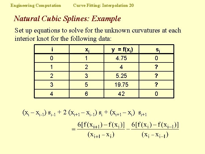
Engineering Computation Curve Fitting: Interpolation 20 Natural Cubic Splines: Example Set up equations to solve for the unknown curvatures at each interior knot for the following data: i xi y = f(xi) si 0 1 4. 75 0 1 2 4 ? 2 3 5. 25 ? 3 5 19. 75 ? 4 6 42 0 (xi – xi-1) si-1 + 2 (xi+1 – xi-1) si + (xi+1 – xi) si+1

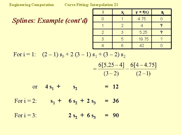
Engineering Computation Curve Fitting: Interpolation 21 Splines: Example (cont'd) For i = 1: xi y = f(xi) 0 1 4. 75 0 1 2 4 ? 2 3 5. 25 ? 3 5 19. 75 ? 4 6 42 0 (2 – 1) s 0 + 2 (3 – 1) s 1 + (3 – 2) s 2 or 4 s 1 + For i = 2: s 1 + For i = 3: i s 2 = 12 6 s 2 + 2 s 3 = 36 2 s 2 + 6 s 3 = 90 si

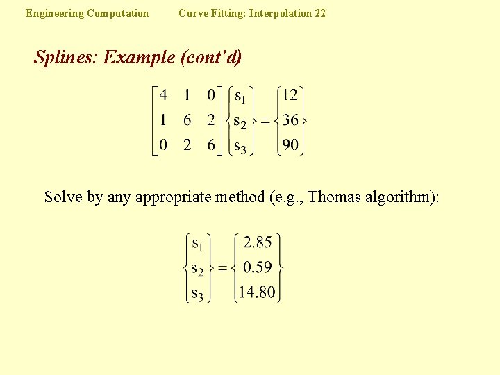
Engineering Computation Curve Fitting: Interpolation 22 Splines: Example (cont'd) Solve by any appropriate method (e. g. , Thomas algorithm):

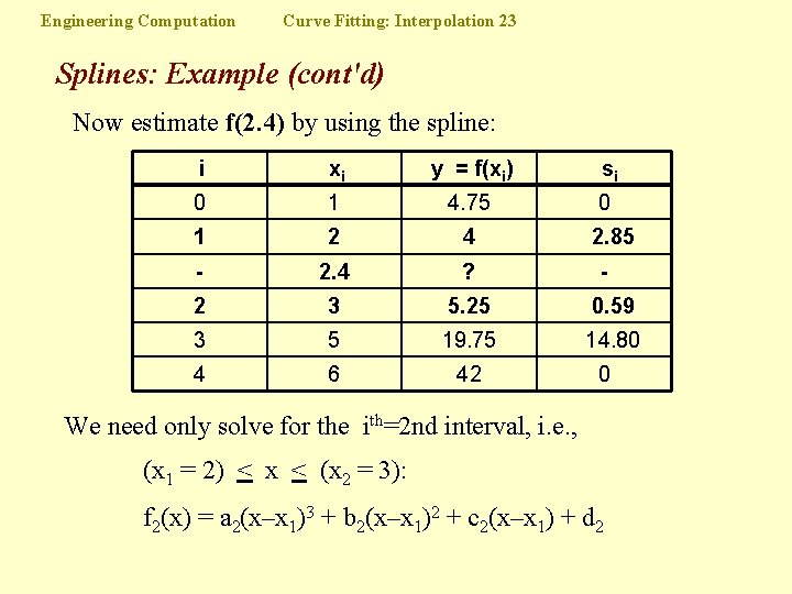
Engineering Computation Curve Fitting: Interpolation 23 Splines: Example (cont'd) Now estimate f(2. 4) by using the spline: i xi y = f(xi) si 0 1 4. 75 0 1 2 4 - 2. 4 ? 2 3 5. 25 0. 59 3 5 19. 75 14. 80 4 6 42 2. 85 - 0 We need only solve for the ith=2 nd interval, i. e. , (x 1 = 2) < x < (x 2 = 3): f 2(x) = a 2(x–x 1)3 + b 2(x–x 1)2 + c 2(x–x 1) + d 2

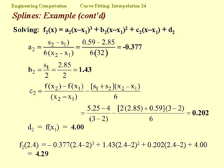
Engineering Computation Curve Fitting: Interpolation 24 Splines: Example (cont'd) Solving: f 2(x) = a 2(x–x 1)3 + b 2(x–x 1)2 + c 2(x–x 1) + d 2 = f(x 1) = 4. 00 f 2(2. 4) = – 0. 377(2. 4– 2)3 + 1. 43(2. 4– 2)2 + 0. 202(2. 4– 2) + 4. 00 = 4. 29

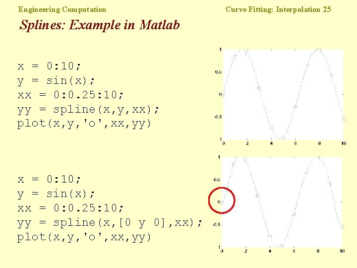
Engineering Computation Splines: Example in Matlab x = 0: 10; y = sin(x); xx = 0: 0. 25: 10; yy = spline(x, y, xx); plot(x, y, 'o', xx, yy) x = 0: 10; y = sin(x); xx = 0: 0. 25: 10; yy = spline(x, [0 y 0], xx); plot(x, y, 'o', xx, yy) Curve Fitting: Interpolation 25

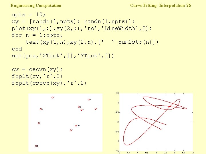
Engineering Computation Curve Fitting: Interpolation 26 npts = 10; xy = [randn(1, npts); randn(1, npts)]; plot(xy(1, : ), xy(2, : ), 'ro', 'Line. Width', 2); for n = 1: npts, text(xy(1, n), xy(2, n), [' ' num 2 str(n)]) end set(gca, 'XTick', [], 'YTick', []) cv = cscvn(xy); fnplt(cv, 'r', 2) fnplt(cscvn(xy), 'r', 2)