ANKARA UNIVERSITY DEPARTMENT OF ENERGY ENGINEERING NUMERICAL METHODS

ANKARA UNIVERSITY DEPARTMENT OF ENERGY ENGINEERING NUMERICAL METHODS INSTRUCTOR DR. ÖZGÜR SELİMOĞLU

CONTENTS Ø Finding roots of equations a) Systems of equations b) Zeros of Polynomials c) Other Methods

SYSTEMS OF EQUATIONS To this point, we have focused on the determination of the roots of a single equation. A related problem is to locate the roots of a set of simultaneous equations, (1) The solution of this system consists of a set of x values that simultaneously result in all the equations equaling zero. Present methods for the case where the simultaneous equations are linear—that is, they can be expressed in the general form; (2) where the b and the a’s are constants. Algebraic and transcendental equations that do not fit this format are called nonlinear equations. For example, are two simultaneous nonlinear equations with two unknowns, x and y. They can be expressed in the form of Eq. (1) as (3. a) (3. b)

Thus, the solution would be the values of x and y that make the functions u(x, y) and v(x, y) equal to zero. Most approaches for determining such solutions are extensions of the open methods for solving single equations. In this section, we will investigate two of these: fixed-point iteration and Newton-Raphson. Ø Fixed-Point Iteration The fixed-point-iteration approach can be modified to solve two simultaneous, nonlinear equations. This approach will be illustrated in the following example. Problem Statement: Use fixed-point iteration to determine the roots of Eq. (3). Note that a correct pair of roots is x = 2 and y = 3. Initiate the computation with guesses of x = 1. 5 and y = 3. 5. Solution: Equation (3. a) can be solved for (4) and Eq. (3. b) can be solved for (5) Note that we will drop the subscripts for the remainder of the example. On the basis of the initial guesses, Eq. (4) can be used to determine a new value of x: This result and the initial value of y = 3. 5 can be substituted into Eq. (5) to determine a new value of y:

Thus, the approach seems to be diverging. This behavior is even more pronounced on the second iteration: Obviously, the approach is deteriorating. Now we will repeat the computation but with the original equations set up in a different format. For example, an alternative formulation of Eq. (3. a) is and of Eq. (3. b) is Now the results are more satisfactory: Thus, the approach is converging on the true values of x = 2 and y = 3.

Example 1: Use fixed-point iteration to determine the roots of x 2 -x – 1=0. That a correct of root is x = 2. Solution: f(x) x 2 -x – 1=0 g(x) x=1+1/x 1 =2 2 x 2 = 1+1/x 1=1+1/2=1. 5 3 x 3 =1+1/x 2=1+1/1. 5=1. 6666 4 x 4 =1+1/x 3=1+1/1. 6666=1. 6 5 x 5 =1+1/x 4=1+1/1. 6=1. 625 6 x 6 =1+1/x 5=1+1/1. 625=1. 615385 7 x 7 =1+1/x 6=1+1/1. 615385=1. 619 8 x 8 =1+1/x 7=1+1/1. 619=1. 6176 9 x 9 =1+1/x 8=1+1/1. 6176=1. 61819 10 x 10 =1+1/x 9=1+1/1. 61819=1. 6179

x 1=g 1(y 0) ln(1 -0)=ln(1) 0 y 1=g 1(x 0) -2 x 2=g 2(y 1) ln(1 -(-2))=ln(3) 1, 0986 y 2=g 2(x 1) -1, 671 x 3=g 3(y 2) ln(1 -(-1, 671))=ln(1) 0, 9824 y 3=g 3(x 2) -1, 7421 x 4=g 4(y 3) ln(1 -(-1, 7421))=ln(2, 7421) 1, 008724 y 4=g 4(x 3) -1, 727 The solution is converging to the exact solution of x=1. 004169 , y= - 1. 729637

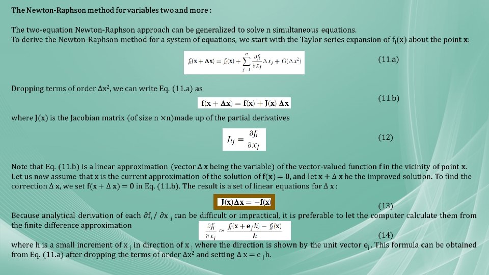
Ø Newton-Raphson Recall that the Newton-Raphson method was predicated on employing the derivative (that is, the slope) of a function to estimate its intercept with the axis of the independent variable. (6) where xi is the initial guess at the root and xi+1 is the point at which the slope intercepts the x axis. At this intercept, f(xi+1) by definition equals zero and Eq. (6) can be rearranged to yield (7) The multi-equation form is derived in an identical fashion. However, a multivariable Taylor series must be used to account for the fact that more than one independent variable contributes to the determination of the root. For the two-variable case, a first-order Taylor series can be written for each nonlinear equation as (8. a) And (9. b) Just as with fixed-point iteration, the Newton-Raphson approach will often diverge if the initial guesses are not sufficiently close to the true roots. Although there are some advanced approaches for obtaining acceptable first estimates, often the initial guesses must be obtained on the basis of «trial and error» and knowledge of the physical system being modeled.

f 1=ui f 3=vi f 1=vi f 3=ui

Example 3: Use the multiple-equation Newton-Raphson method to determine roots of Eq. (a, b). Note that a correct pair of roots is x = 2 and y = 3. Initiate the computation with guesses of x = 1. 5 and y = 3. 5. (a) (b) Solution: First compute the partial derivatives and evaluate them at the initial guesses of x and y: Thus, the determinant of the Jacobian matrix for the first iteration is The values of the functions can be evaluated at the initial guesses as These values can be substituted into Eq. (10) to give Thus, the results are converging to the true values of x = 2 and y = 3. The computation can be repeated until an acceptable accuracy is obtained.

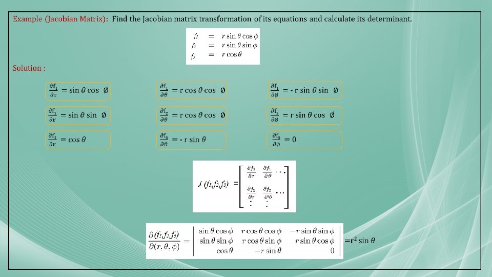
The Jacobian Matrix In the vector calculation, the Jacobi matrix is the matrix containing all first-order partial derivatives of a vector-valued function. When this matrix is a square matrix, that is, if the number of inputs of the function is the same as the vector components of the output number, the determinant of this matrix is called the Jacobi determinant. A system of nonlinear equations has the form Equations matrix (a) Define the matrix J(x) by. The matrix J is the derivative of the F matrix according to its variables. (b)

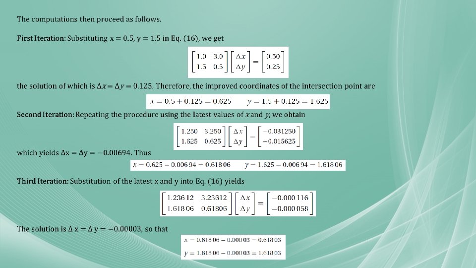
By plotting the circle and the hyperbola , we see that there are four points of intersection. It is sufficient, however, to find only one of these points, because the others can be deduced from symmetry. From the plot we also get a rough estimate of the coordinates of an intersection point, x = 0. 5, y = 1. 5, which we use as the starting values.

Subsequent iterations would not change the results within five significant figures. Therefore, the coordinates of the four intersection points are Alternate Solution: If there are only a few equations, it may be possible to eliminate all but one of the unknowns. Then we would be left with a single equation that can be solved by the methods described. which upon substitution into Eq. (16) yields x 2 + 1/x 2 − 3 = 0, or The solutions of this biquadratic equation are x = ± 0. 618 03 and ± 1. 618 03, which agree with the results obtained by the Newton. Raphson method.

OTHER METHOD Ø BRENT’S METHOD Inverse Quadratic Interpolation Inverse quadratic interpolation is similar to the secant method. As in Fig. 1. a, the secant method is based on computing a straight line that goes through two guesses. The intersection of this straight line with the x axis represents the new root estimate. For this reason, it is sometimes referred to as a linear interpolation method. Now suppose that we had three points. In that case, we could determine a quadratic function of x that goes through the three points (Fig. 1. b). Just as with the linear secant method, the intersection of this parabola with the x axis would represent the new root estimate. And as illustrated in Fig. 1. b, using a curve rather than a straight line often yields a better estimate. Figure 1: Comparison of (a) the secant method and (b) inverse quadratic interpolation. Note that the dark parabola passing through the three points in (b) is called “inverse” because it is written in y rather than in x.

The difficulty can be rectified by employing inverse quadratic interpolation. That is, rather than using a parabola in x, we can fit the points with a parabola in y. This amounts to reversing the axes and creating a “sideways” parabola (the curve, x = f (y), in Fig. 2). If the three points are designated as (xi− 2, yi− 2), (xi− 1, yi− 1), and (xi , yi ), a quadratic function of y that passes through the points can be generated as (17) The root, xi+1, corresponds to y = 0, which when substituted into Eq. (6. 9) yields (18) As shown in Fig. 2, such a “sideways” parabola always intersects the x-axis. Figure 2: Two parabolas fit to three points. The parabola written as a function of x, y = f(x), has complex roots and hence does not intersect the x axis. In contrast, if the variables are reversed, and the parabola developed as x = f (y), the function does intersect the x axis.

Example 5: Develop quadratic equations in both x and y for the data points depicted in Fig. : (1, 2), (2, 1), and (4, 5). For the first, y = f (x), employ the quadratic formula to illustrate that the roots are complex. For the latter, x = g(y), use inverse quadratic interpolation (Eq. 10) to determine the root estimate. Solution: By reversing the x’s and y’s, Eq. (17) can be used to generate a quadratic in x as or collecting terms This equation was used to generate the parabola, y = f(x), in Fig.

The quadratic formula can be used to determine that the roots for this case are complex, Equation (17) can be used to generate the quadratic in y as or collecting terms Finally, Eq. (6. 10) can be used to determine the root as

Ø REFERENCES • Jaan Kiusalaas, “Numerical Methods in Engineering with Python 3”, 3 rd Edition, Cambridge, NY, 2013 • S. C. Chapra and R. P. Canale, “Numerical Methods for Engineers”, 6 th ed. , Mc. Graw-Hill, NY, 2010