Numerical Optimization Techniques For Engineering Design By G

Numerical Optimization Techniques For Engineering Design By: G. N. Vanderplaat • Optimization Theory And Applications By : S. S. Rao • An Introduction To Optimization By : E. K. P. Chong & S. H. Zak • Applied Optimization with MATLAB Programming By : P. Venkataraman •

NUMERICAL OPTIMIZATION TECHNIQUES

OPTIMIZATION METHODS Any problem with several solutions can be considered as an optimization problem 1 -Experimental Optimization 2 -Analytical Optimization 3 -Numerical Optimization

Parameters in Optimization 1 -Objective Function 2 -Design Variables 3 -Constraints local Optimum point Global Optimum

Optimization Problems

Numerical Optimization Methods Ø Zero order Ø Classic Methods Ø First order Ø Second order Ø Heuristic Methods

Unconstrained Problem Step 1: Step 2:

Step 3: if hessian matrix P. D X* min if hessian matrix N. D X* max

Example Assume we wish to find the minimum value of the following algebraic function F(X) is referred to as the objective function is to be minimized, and we wish to determine the combination of the variables X 1 and X 2 , and we call them the design, or decision, variables.

No limited are imposed on the values of X 1 and X 2 and no additional conditions must be met for the “design” to be acceptable. Therefore, F(X) is said to be unconstrained We know from basic calculus that at the optimum, or minimum, of F(X), the partial derivatives with respect to X 1 and X 2 must vanish. That is Solving for X 1 and X 2 , we find that indeed X 1*=1 and X 2*=1.

Ø H at (1, 1) is positive definite so the extremum is minimum

Optimum point is at X 1*=1 and X 2*=1.

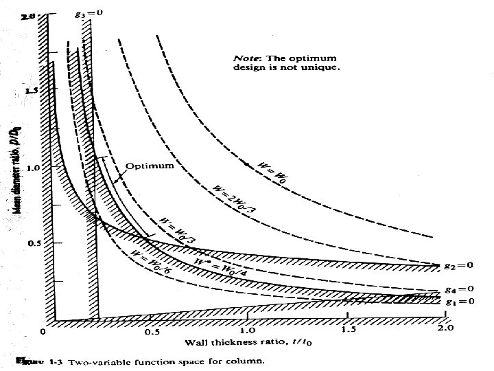
Constrained function minimization Example Figure 1 -2 a depicts a tubular column of height h which is required to support a concentrated load P as shown we wish to find the mean diameter D and the wall thickness t to minimize the weight of column.

Objective Function : Where A is the cross-sectional area and ρ is the material , s unite weight. Design Variable : D , t call design variable. Constraints : E = Young modulus I = moment of inertial ν = poisson ratio

normalizing

General Problem Statement We can now write the nonlinear constrained optimization problem mathematically as follows:

The Iterative Optimization Procedure Most optimization algorithms require that an initial set of design variable, X 0 , be specified Beginning from this starting point, the design is updated iteratively. Probably the most common form of this iterative procedure is given by : Where q is the iteration number and S is vector search direction in the design space. The scalar quantity α* defines the distance that we wish to move in direction S.

Optimum point Local Optimum Ø Global Optimum Ø Ø Only in CONVEX problems the optimum point is GLOBAL. If Hessian matrix of a function is positive definite, the function is convex function. Ø If objective function and all constraints are convex, then the problem is convex. Ø In convex problems, K-T conditions are necessary and sufficient conditions for optimum. Ø

Search in direction S

Constrained Problem

Example:

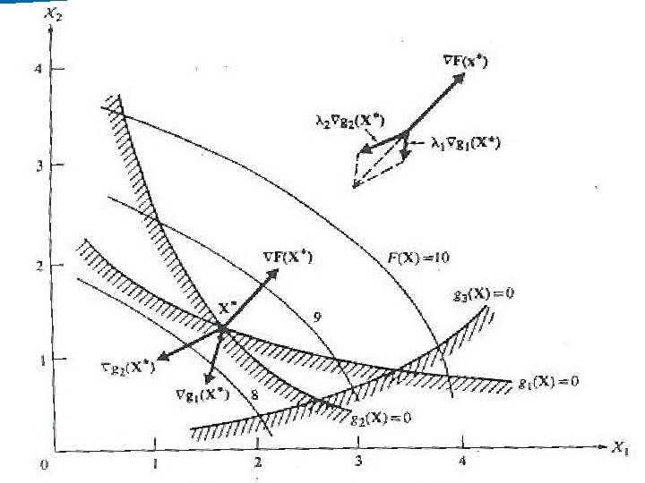
The Kuhn-Tucker Conditions The necessary conditions for optimum point :

Ø At the optimum point :

Example: