Chem 302 Math 252 Chapter 3 Interpolation Extrapolation

Chem 302 - Math 252 Chapter 3 Interpolation / Extrapolation

Interpolation / Extrapolation • Experimental data at discrete points • Need to know the dependent variable at a value of the independent variable that was not measured • Need to know what value of the independent variable gives a particular value of the dependent variable • Point is within range of experimental data then called interpolation • Point is outside range of experimental data then call extrapolation • Same techniques • Extrapolation more risky

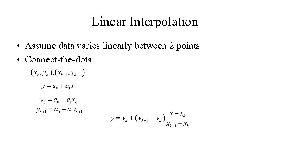
Linear Interpolation • Assume data varies linearly between 2 points • Connect-the-dots

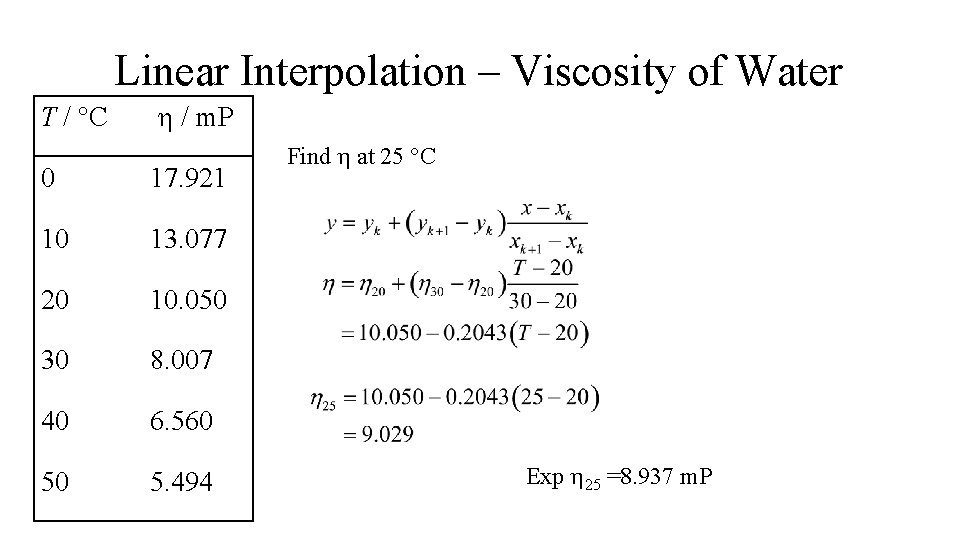
Linear Interpolation – Viscosity of Water T / °C / m. P 0 17. 921 10 13. 077 20 10. 050 30 8. 007 40 6. 560 50 5. 494 Find at 25 °C Exp 25 =8. 937 m. P

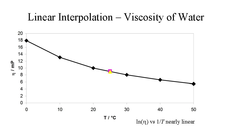
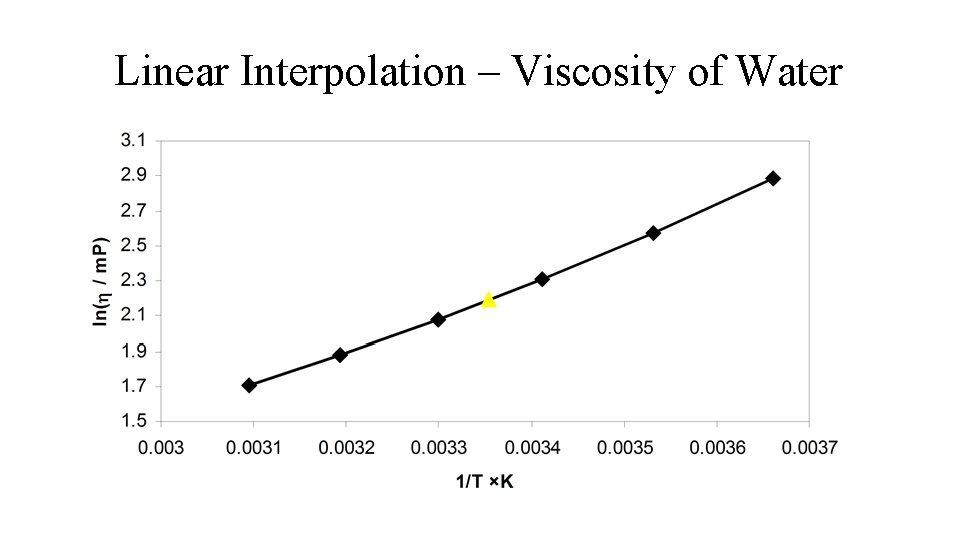
Linear Interpolation – Viscosity of Water ln( ) vs 1/T nearly linear

Linear Interpolation – Viscosity of Water

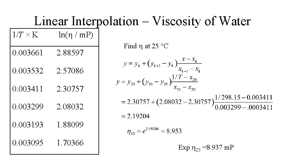
Linear Interpolation – Viscosity of Water 1/T × K ln( / m. P) 0. 003661 2. 88597 0. 003532 2. 57086 0. 003411 2. 30757 0. 003299 2. 08032 0. 003193 1. 88099 0. 003095 1. 70366 Find at 25 °C Exp 25 =8. 937 m. P

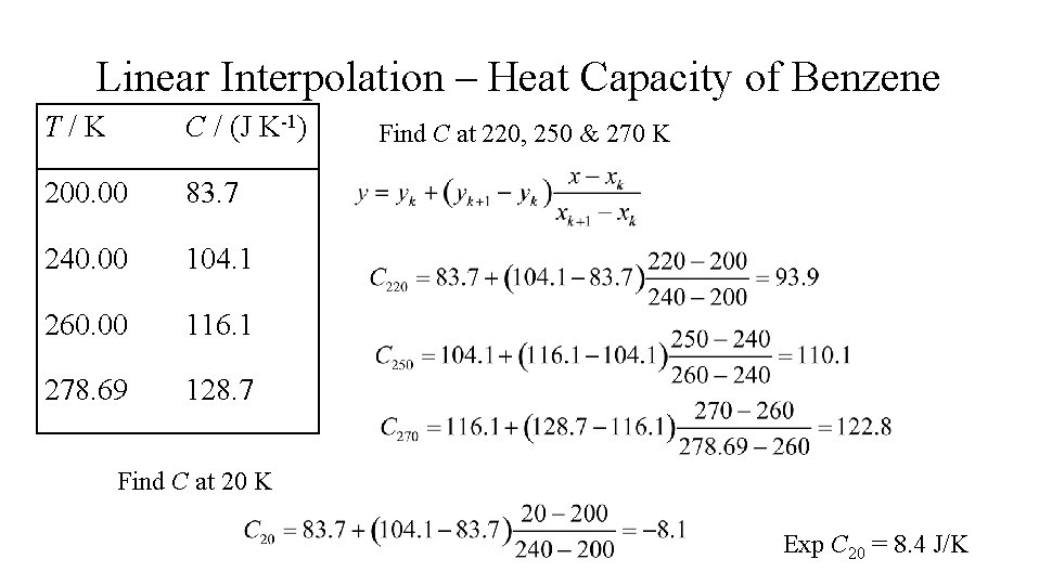
Linear Interpolation – Heat Capacity of Benzene T/K C / (J K-1) 200. 00 83. 7 240. 00 104. 1 260. 00 116. 1 278. 69 128. 7 Find C at 220, 250 & 270 K Find C at 20 K Exp C 20 = 8. 4 J/K

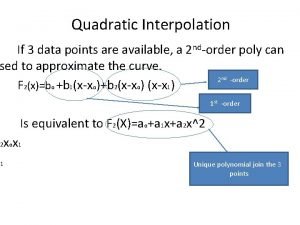
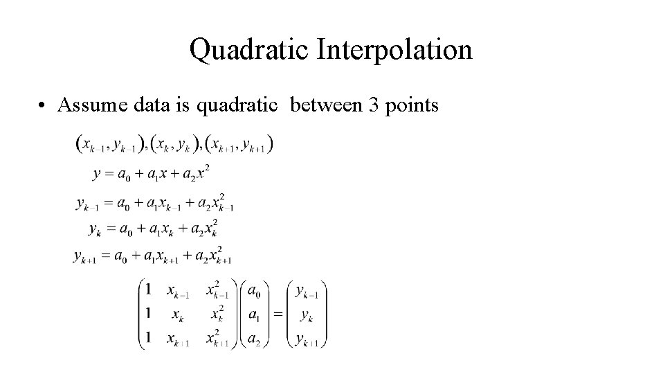
Quadratic Interpolation • Assume data is quadratic between 3 points

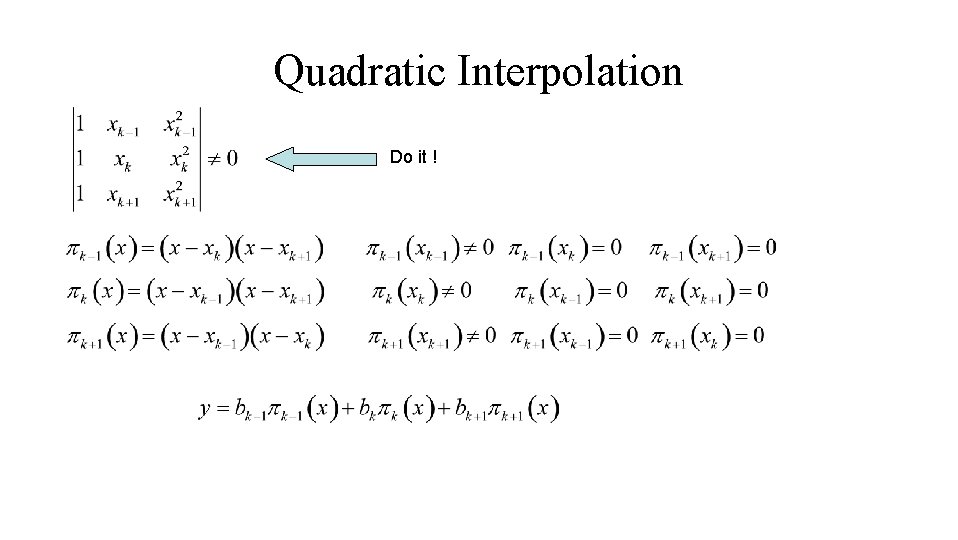
Quadratic Interpolation Do it !

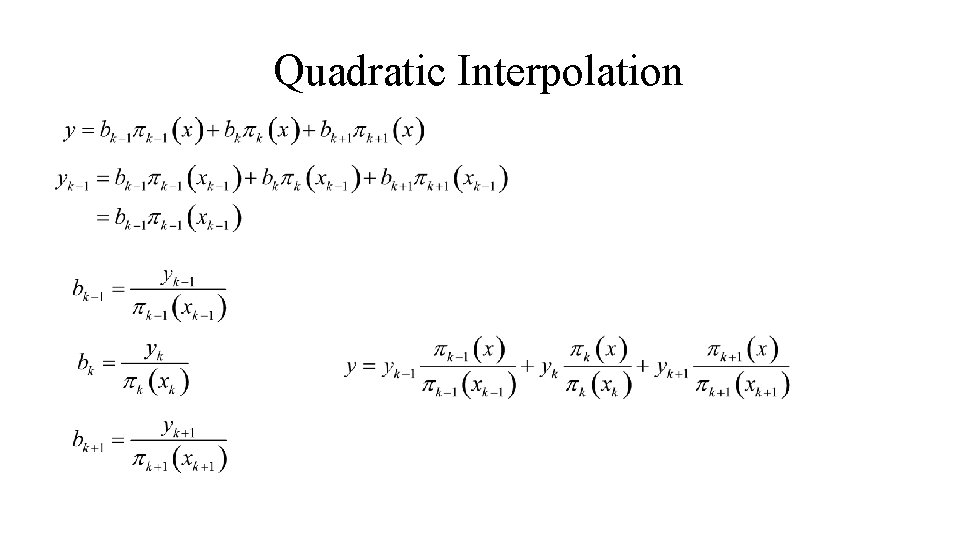
Quadratic Interpolation

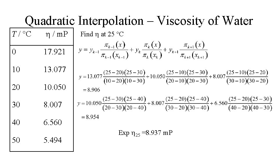
Quadratic Interpolation – Viscosity of Water T / °C / m. P 0 17. 921 10 13. 077 20 10. 050 30 8. 007 40 6. 560 50 5. 494 Find at 25 °C Exp 25 =8. 937 m. P

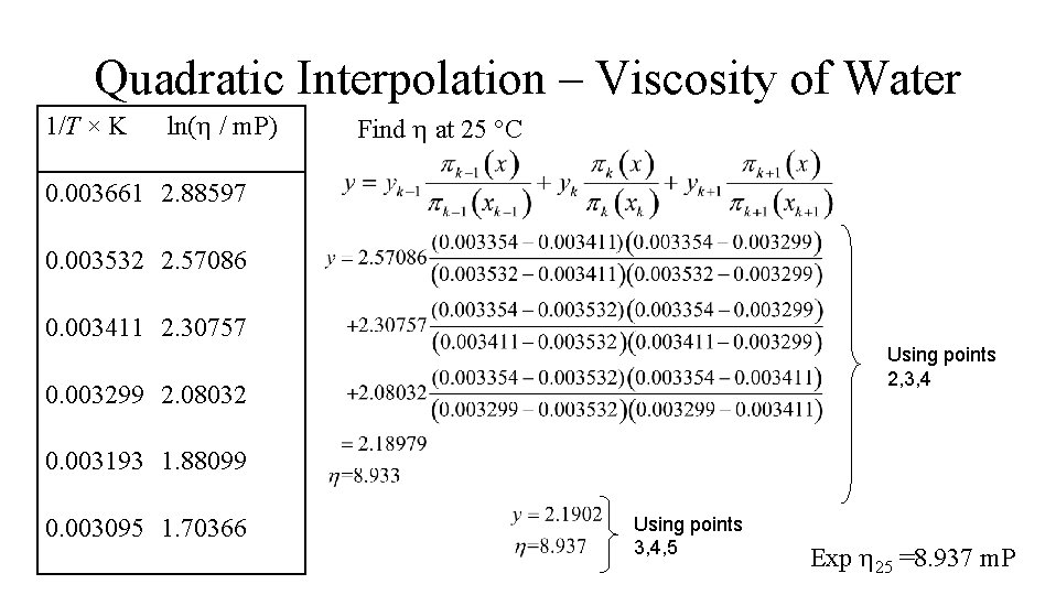
Quadratic Interpolation – Viscosity of Water 1/T × K ln( / m. P) Find at 25 °C 0. 003661 2. 88597 0. 003532 2. 57086 0. 003411 2. 30757 Using points 2, 3, 4 0. 003299 2. 08032 0. 003193 1. 88099 0. 003095 1. 70366 Using points 3, 4, 5 Exp 25 =8. 937 m. P

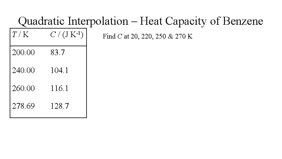
Quadratic Interpolation – Heat Capacity of Benzene T/K C / (J K-1) 200. 00 83. 7 240. 00 104. 1 260. 00 116. 1 278. 69 128. 7 Find C at 20, 250 & 270 K

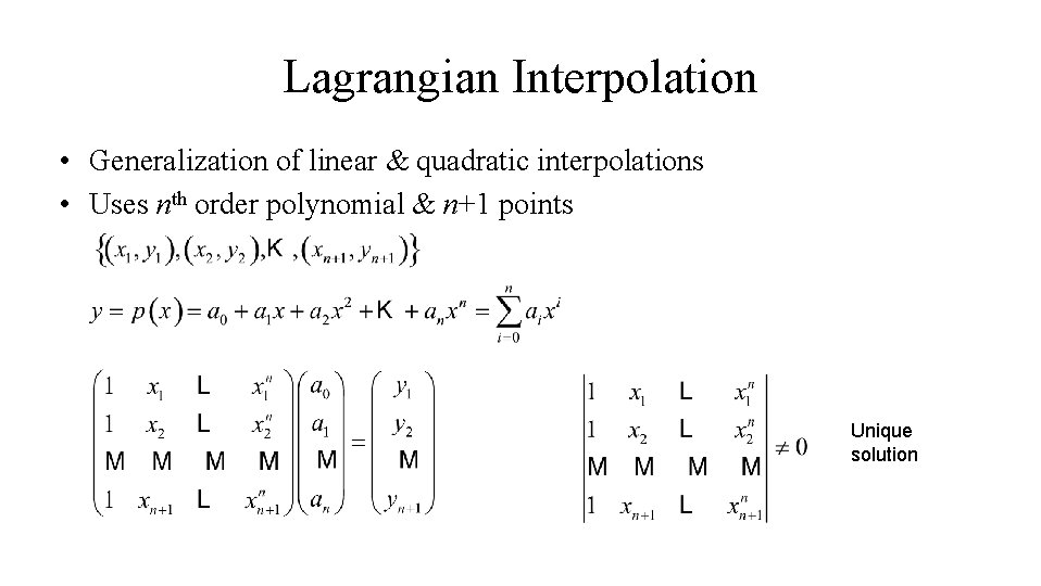
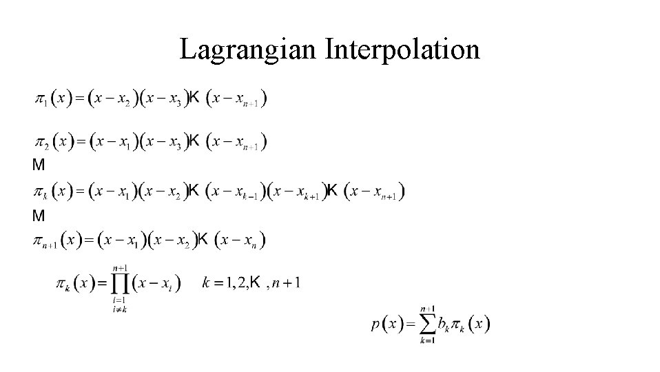
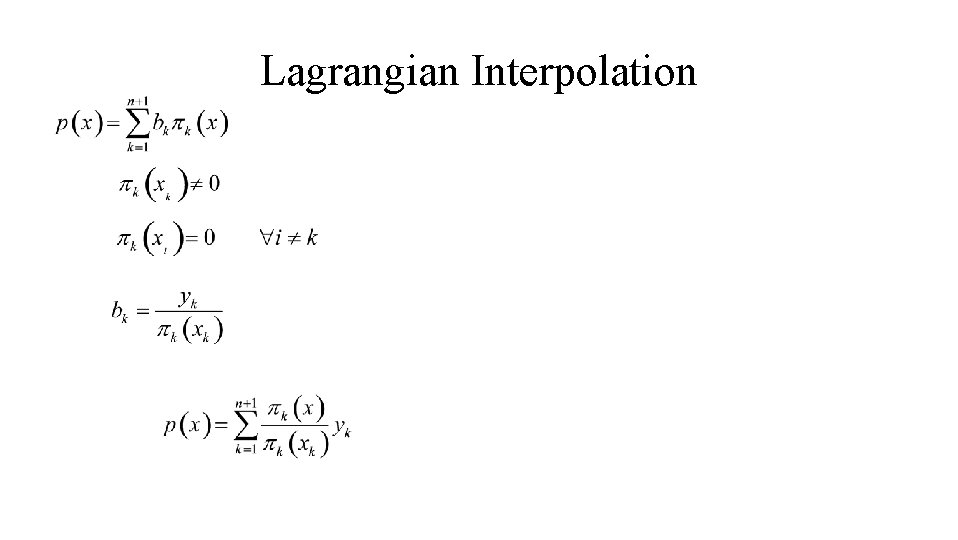
Lagrangian Interpolation • Generalization of linear & quadratic interpolations • Uses nth order polynomial & n+1 points Unique solution

Lagrangian Interpolation

Lagrangian Interpolation

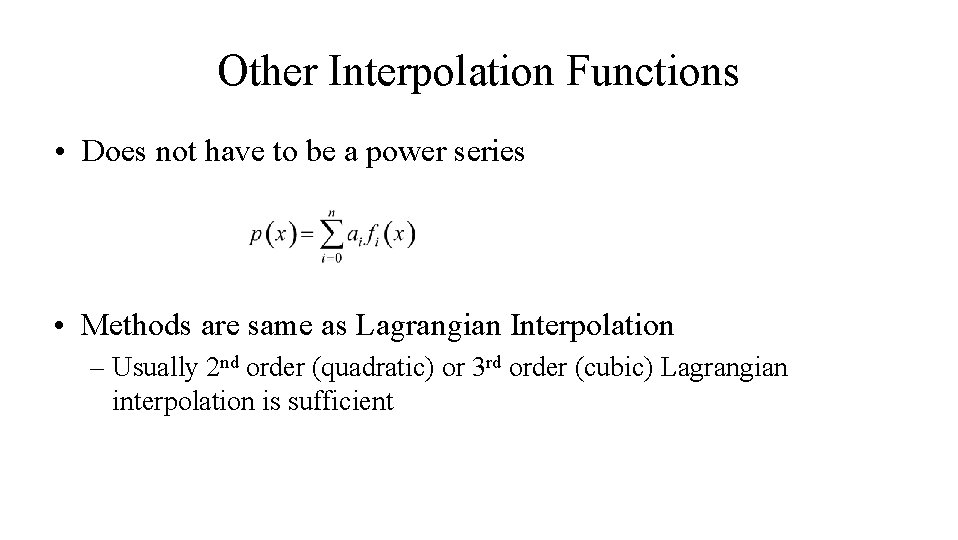
Other Interpolation Functions • Does not have to be a power series • Methods are same as Lagrangian Interpolation – Usually 2 nd order (quadratic) or 3 rd order (cubic) Lagrangian interpolation is sufficient

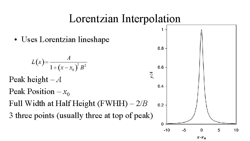
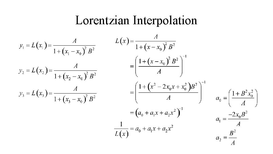
Lorentzian Interpolation • Uses Lorentzian lineshape Peak height – A Peak Position – x 0 Full Width at Half Height (FWHH) – 2/B 3 three points (usually three at top of peak)

Lorentzian Interpolation

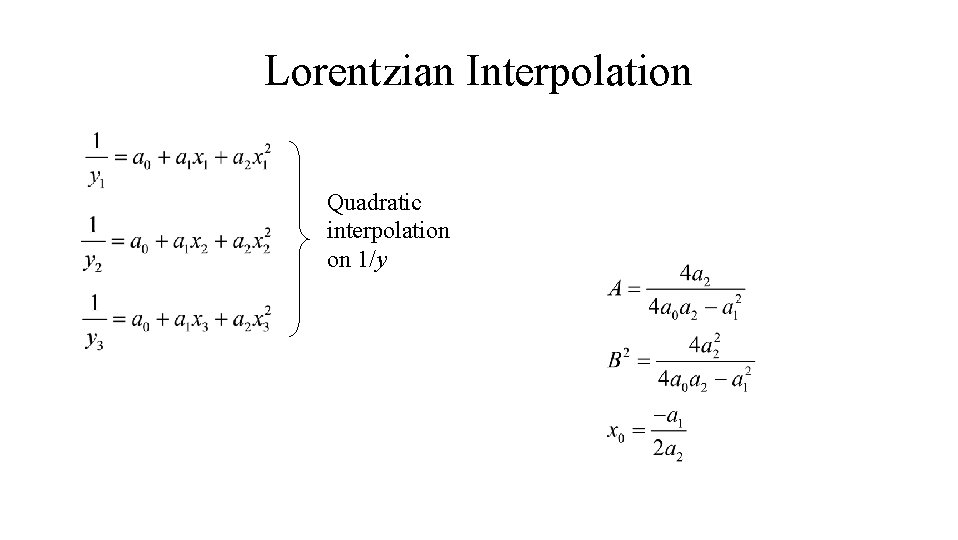
Lorentzian Interpolation Quadratic interpolation on 1/y

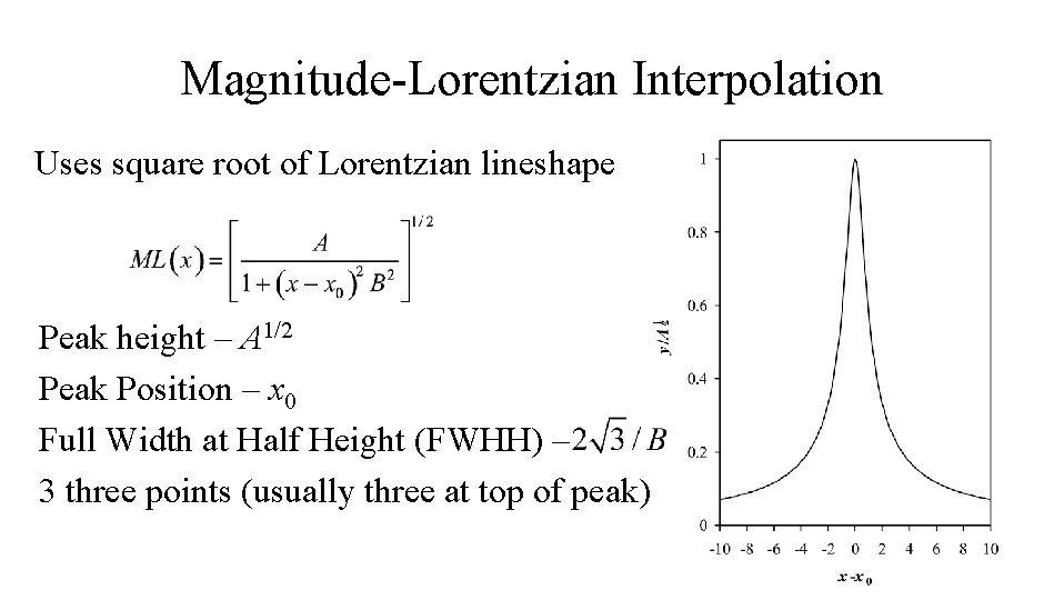
Magnitude-Lorentzian Interpolation Uses square root of Lorentzian lineshape Peak height – A 1/2 Peak Position – x 0 Full Width at Half Height (FWHH) – 3 three points (usually three at top of peak)

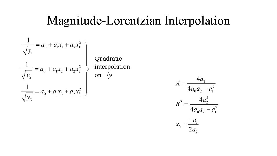
Magnitude-Lorentzian Interpolation Quadratic interpolation on 1/y

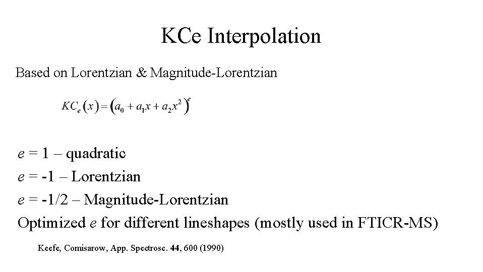
KCe Interpolation Based on Lorentzian & Magnitude-Lorentzian e = 1 – quadratic e = -1 – Lorentzian e = -1/2 – Magnitude-Lorentzian Optimized e for different lineshapes (mostly used in FTICR-MS) Keefe, Comisarow, App. Spectrosc. 44, 600 (1990)

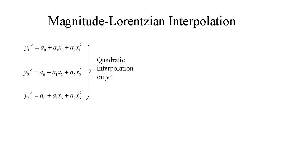
Magnitude-Lorentzian Interpolation Quadratic interpolation on y-e

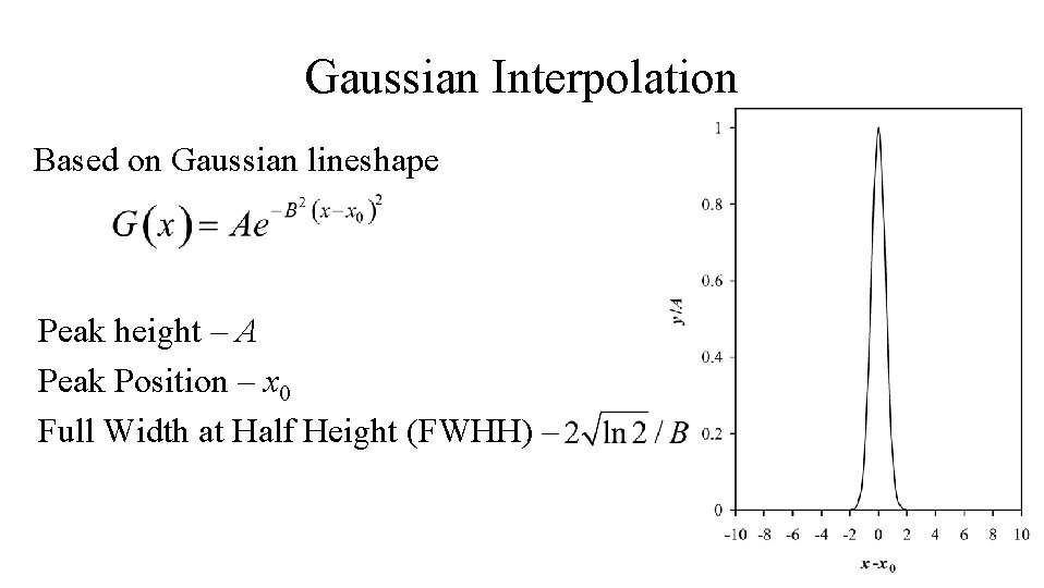
Gaussian Interpolation Based on Gaussian lineshape Peak height – A Peak Position – x 0 Full Width at Half Height (FWHH) –

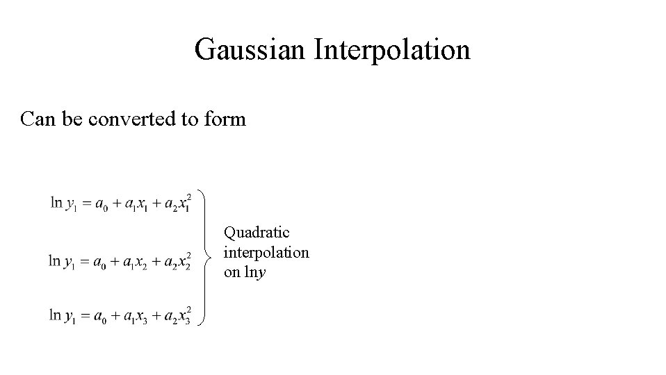
Gaussian Interpolation Can be converted to form Quadratic interpolation on lny

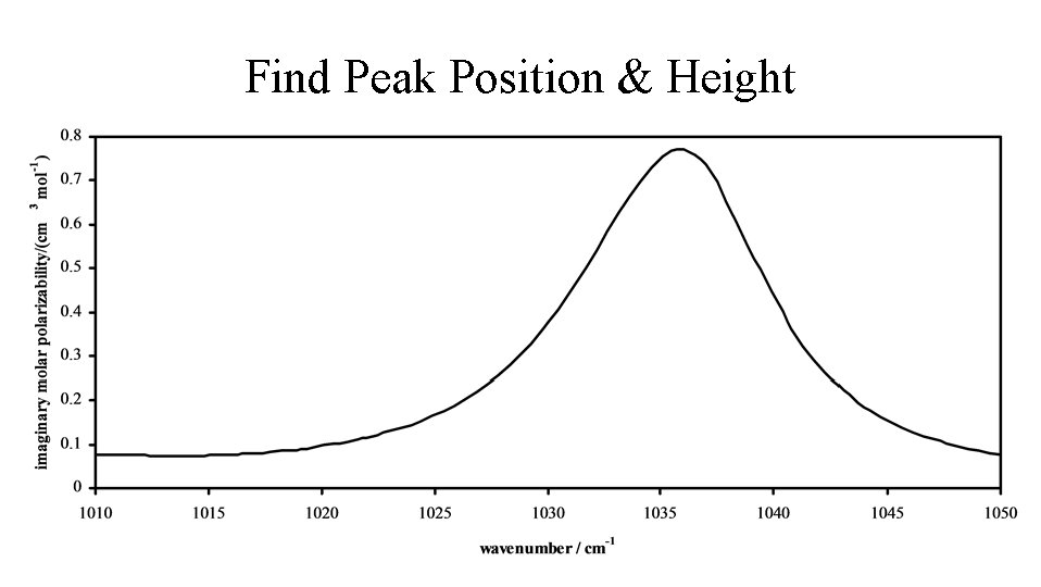
Find Peak Position & Height

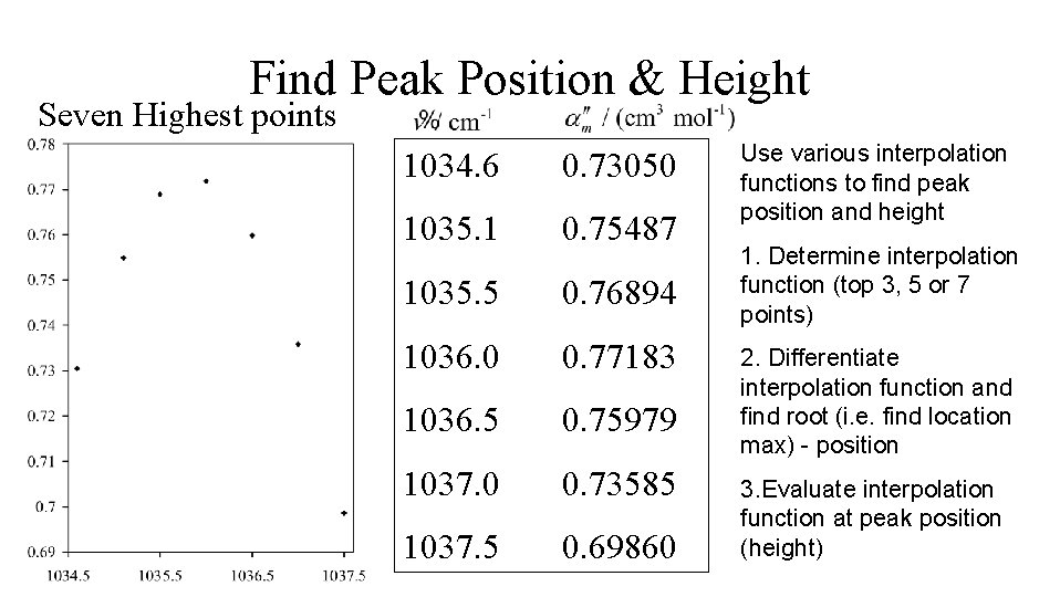
Find Peak Position & Height Seven Highest points 1034. 6 0. 73050 1035. 1 0. 75487 1035. 5 0. 76894 1036. 0 0. 77183 1036. 5 0. 75979 1037. 0 0. 73585 1037. 5 0. 69860 Use various interpolation functions to find peak position and height 1. Determine interpolation function (top 3, 5 or 7 points) 2. Differentiate interpolation function and find root (i. e. find location max) - position 3. Evaluate interpolation function at peak position (height)

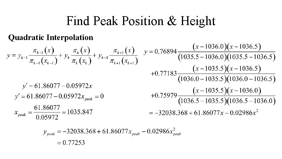
Find Peak Position & Height Quadratic Interpolation

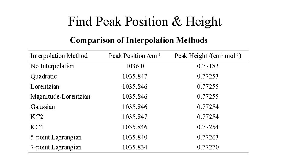
Find Peak Position & Height Comparison of Interpolation Methods Interpolation Method Peak Position /cm-1 Peak Height /(cm 3 mol-1) 1036. 0 0. 77183 Quadratic 1035. 847 0. 77253 Lorentzian 1035. 846 0. 77255 Magnitude-Lorentzian 1035. 846 0. 77255 Gaussian 1035. 846 0. 77254 KC 2 1035. 847 0. 77254 KC 4 1035. 846 0. 77254 5 -point Lagrangian 1035. 840 0. 77263 7 -point Lagrangian 1035. 834 0. 77270 No Interpolation

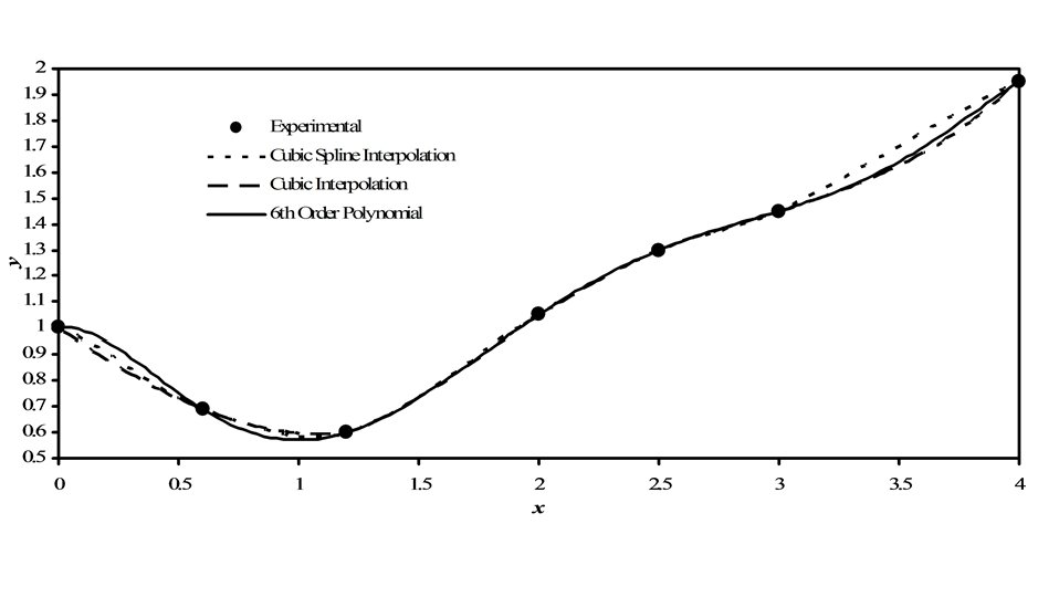
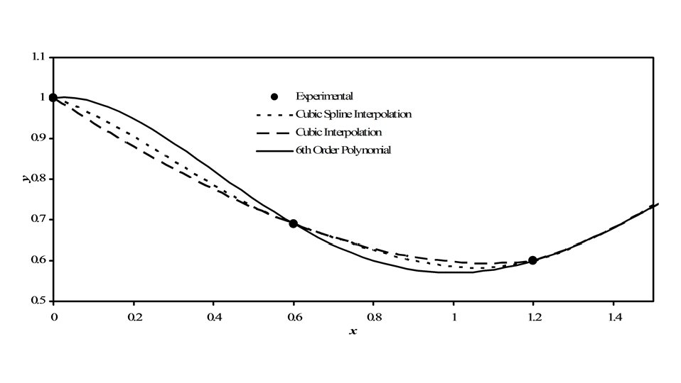
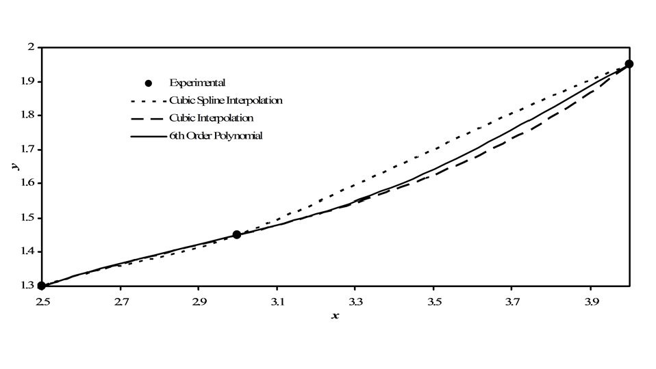
Spline Interpolation • So far methods have used a moving window of subset of data – May be discontinuous at edges of windows – Causes jagged plots • Spline interpolation forces slopes (and in some cases higher derivatives) to match at edges of windows – Creates smooth plots

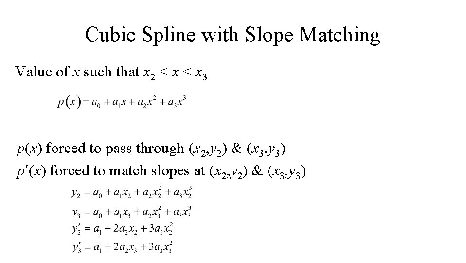
Cubic Spline with Slope Matching Value of x such that x 2 < x 3 p(x) forced to pass through (x 2, y 2) & (x 3, y 3) p (x) forced to match slopes at (x 2, y 2) & (x 3, y 3)

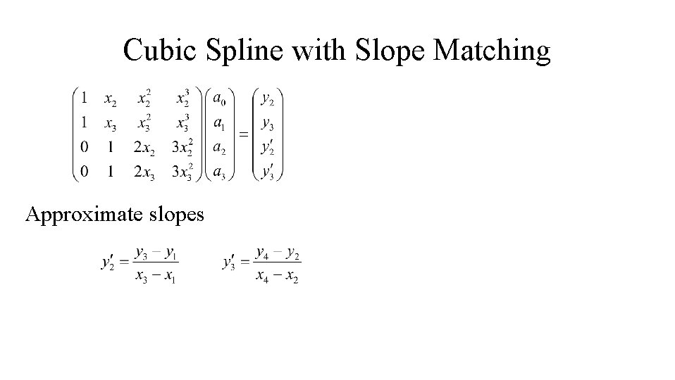
Cubic Spline with Slope Matching Approximate slopes

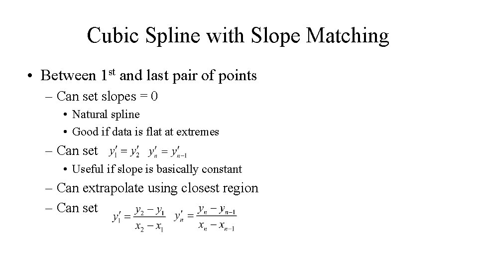
Cubic Spline with Slope Matching • Between 1 st and last pair of points – Can set slopes = 0 • Natural spline • Good if data is flat at extremes – Can set • Useful if slope is basically constant – Can extrapolate using closest region – Can set