CHAPTER 3 NUMERICAL DESCRIPTIVE MEASURES 1 MEASURES OF

CHAPTER 3 NUMERICAL DESCRIPTIVE MEASURES 1

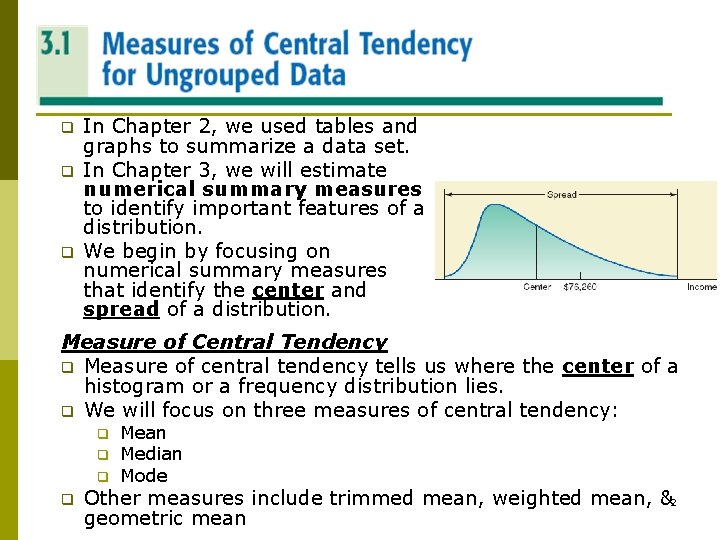
MEASURES OF CENTRAL TENDENCY FOR UNGROUPED DATA q q q In Chapter 2, we used tables and graphs to summarize a data set. In Chapter 3, we will estimate numerical summary measures to identify important features of a distribution. We begin by focusing on numerical summary measures that identify the center and spread of a distribution. Measure of Central Tendency q Measure of central tendency tells us where the center of a histogram or a frequency distribution lies. q We will focus on three measures of central tendency: q q Mean Median Mode Other measures include trimmed mean, weighted mean, &2 geometric mean

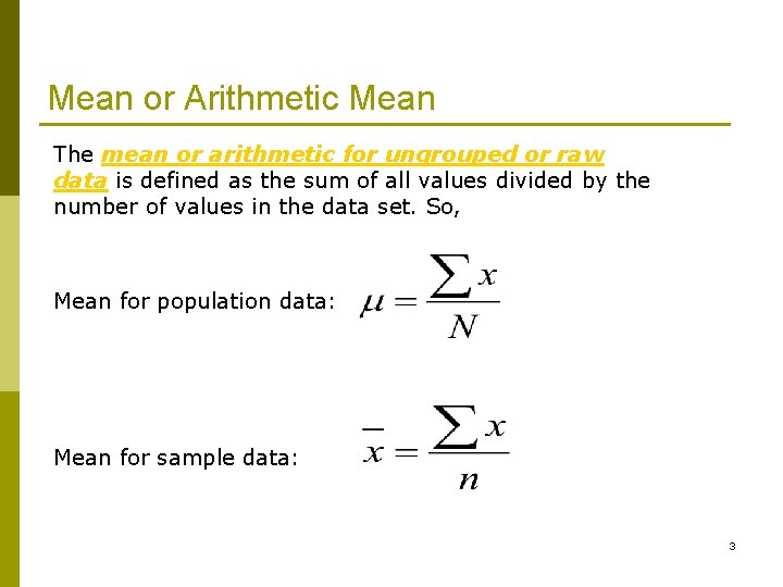
Mean or Arithmetic Mean The mean or arithmetic for ungrouped or raw data is defined as the sum of all values divided by the number of values in the data set. So, Mean for population data: Mean for sample data: 3

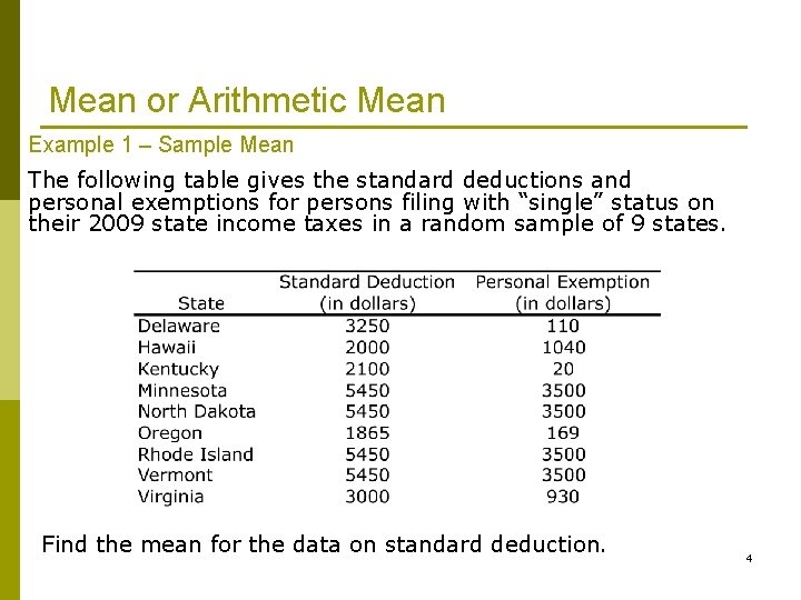
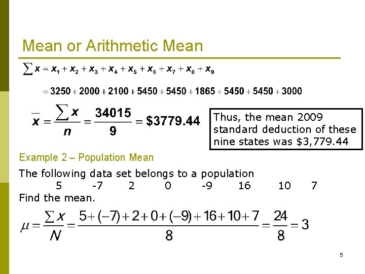
Mean or Arithmetic Mean Example 1 – Sample Mean The following table gives the standard deductions and personal exemptions for persons filing with “single” status on their 2009 state income taxes in a random sample of 9 states. Find the mean for the data on standard deduction. 4

Mean or Arithmetic Mean Thus, the mean 2009 standard deduction of these nine states was $3, 779. 44 Example 2 – Population Mean The following data set belongs to a population 5 -7 2 0 -9 16 Find the mean. 10 7 5

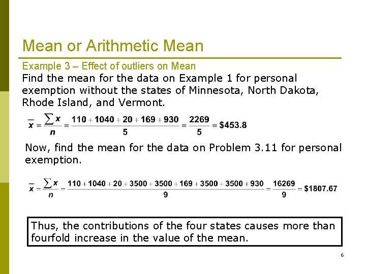
Mean or Arithmetic Mean Example 3 – Effect of outliers on Mean Find the mean for the data on Example 1 for personal exemption without the states of Minnesota, North Dakota, Rhode Island, and Vermont. Now, find the mean for the data on Problem 3. 11 for personal exemption. Thus, the contributions of the four states causes more than fourfold increase in the value of the mean. 6

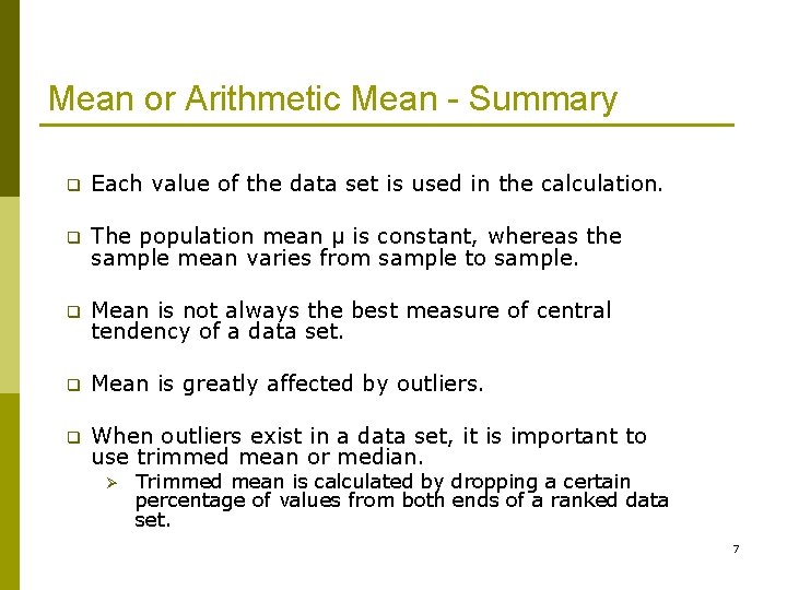
Mean or Arithmetic Mean - Summary q Each value of the data set is used in the calculation. q The population mean µ is constant, whereas the sample mean varies from sample to sample. q Mean is not always the best measure of central tendency of a data set. q Mean is greatly affected by outliers. q When outliers exist in a data set, it is important to use trimmed mean or median. Ø Trimmed mean is calculated by dropping a certain percentage of values from both ends of a ranked data set. 7

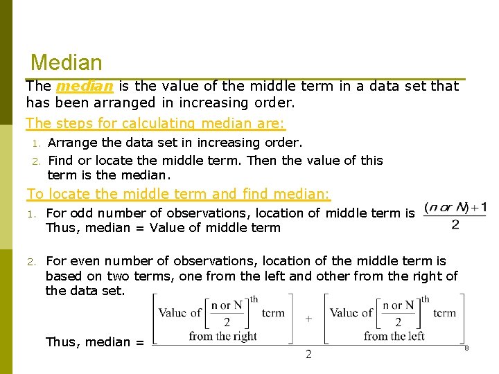
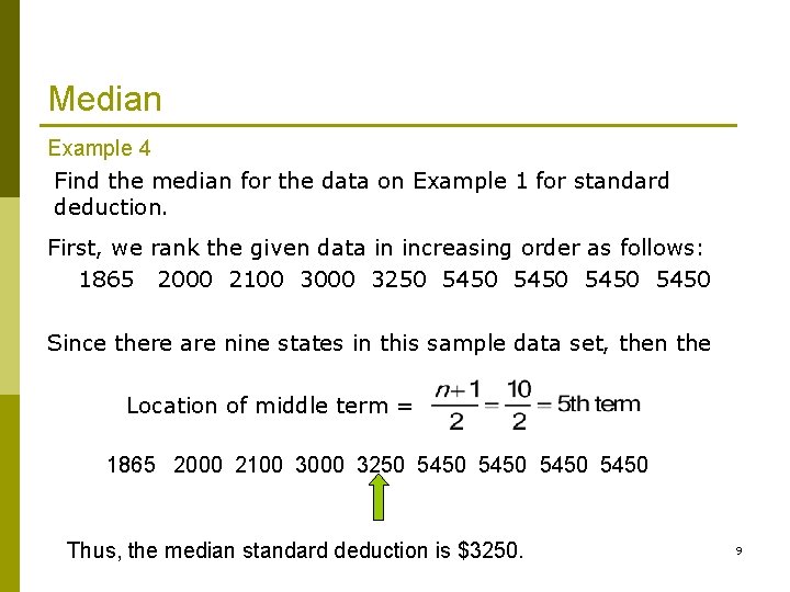
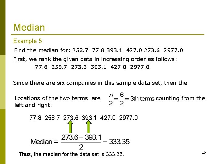
Median The median is the value of the middle term in a data set that has been arranged in increasing order. The steps for calculating median are: 1. 2. Arrange the data set in increasing order. Find or locate the middle term. Then the value of this term is the median. To locate the middle term and find median: 1. For odd number of observations, location of middle term is Thus, median = Value of middle term 2. For even number of observations, location of the middle term is based on two terms, one from the left and other from the right of the data set. Thus, median = 8

Median Example 4 Find the median for the data on Example 1 for standard deduction. First, we rank the given data in increasing order as follows: 1865 2000 2100 3000 3250 5450 Since there are nine states in this sample data set, then the Location of middle term = 1865 2000 2100 3000 3250 5450 Thus, the median standard deduction is $3250. 9

Median Example 5 Find the median for: 258. 7 77. 8 393. 1 427. 0 273. 6 2977. 0 First, we rank the given data in increasing order as follows: 77. 8 258. 7 273. 6 393. 1 427. 0 2977. 0 Since there are six companies in this sample data set, then the Locations of the two terms are left and right. counting from the 77. 8 258. 7 273. 6 393. 1 427. 0 2977. 0 Thus, the median for the data set is 333. 35. 10

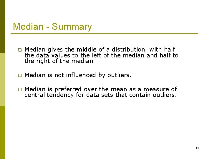
Median - Summary q Median gives the middle of a distribution, with half the data values to the left of the median and half to the right of the median. q Median is not influenced by outliers. q Median is preferred over the mean as a measure of central tendency for data sets that contain outliers. 11

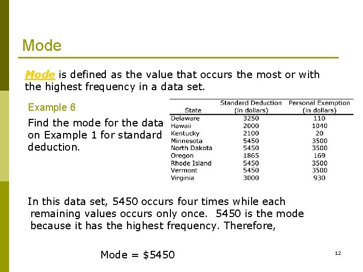
Mode is defined as the value that occurs the most or with the highest frequency in a data set. Example 6 Find the mode for the data on Example 1 for standard deduction. In this data set, 5450 occurs four times while each remaining values occurs only once. 5450 is the mode because it has the highest frequency. Therefore, Mode = $5450 12

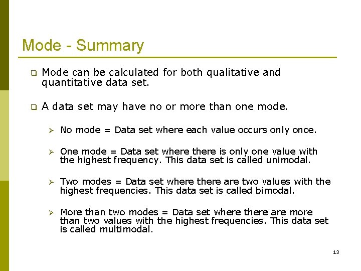
Mode - Summary q Mode can be calculated for both qualitative and quantitative data set. q A data set may have no or more than one mode. Ø No mode = Data set where each value occurs only once. Ø One mode = Data set where there is only one value with the highest frequency. This data set is called unimodal. Ø Two modes = Data set where there are two values with the highest frequencies. This data set is called bimodal. Ø More than two modes = Data set where there are more than two values with the highest frequencies. This data set is called multimodal. 13

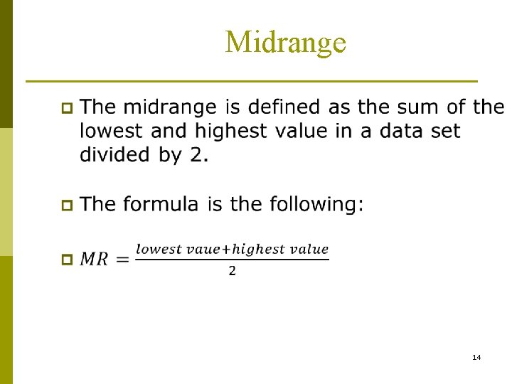
Midrange 14

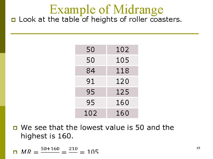
Example of Midrange p Look at the table of heights of roller coasters. 50 50 84 91 102 105 118 120 95 95 102 125 160 15

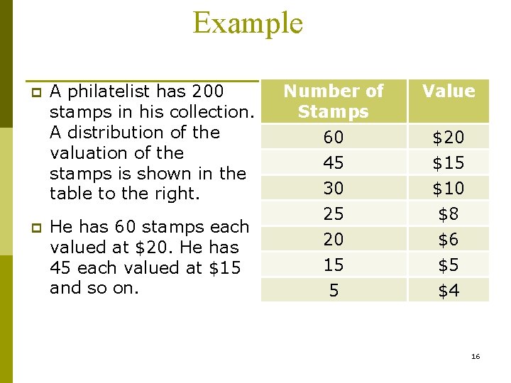
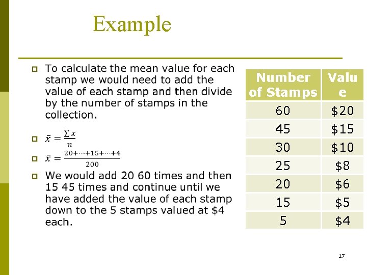
Example p p A philatelist has 200 stamps in his collection. A distribution of the valuation of the stamps is shown in the table to the right. He has 60 stamps each valued at $20. He has 45 each valued at $15 and so on. (1) Number of Stamps 60 45 30 25 20 15 5 Value $20 $15 $10 $8 $6 $5 $4 16

Example (2) Number Valu of Stamps e 60 $20 45 $15 30 $10 25 $8 20 $6 15 $5 5 $4 17

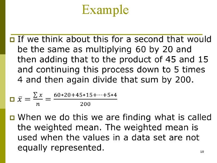
Example (3) 18

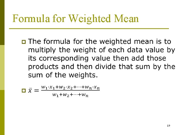
Formula for Weighted Mean 19

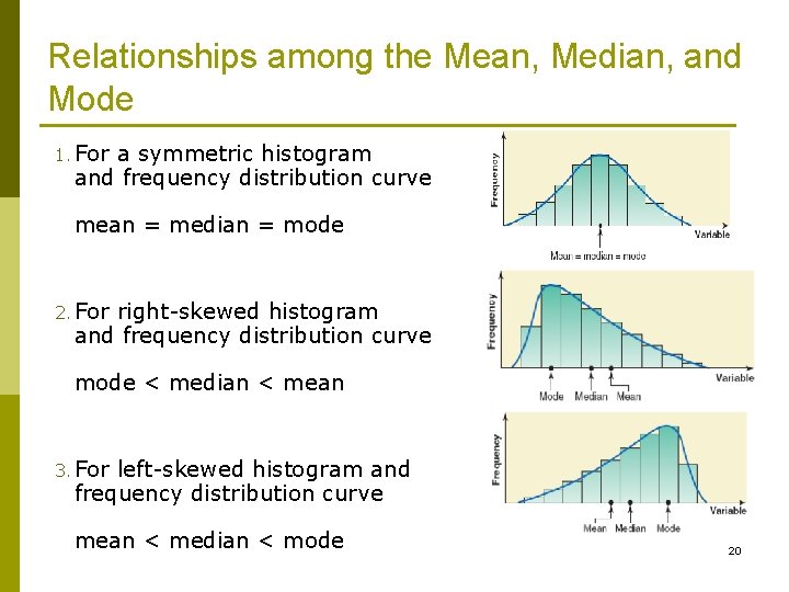
Relationships among the Mean, Median, and Mode 1. For a symmetric histogram and frequency distribution curve mean = median = mode 2. For right-skewed histogram and frequency distribution curve mode < median < mean 3. For left-skewed histogram and frequency distribution curve mean < median < mode 20

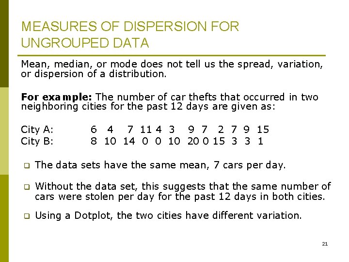
MEASURES OF DISPERSION FOR UNGROUPED DATA Mean, median, or mode does not tell us the spread, variation, or dispersion of a distribution. For example: The number of car thefts that occurred in two neighboring cities for the past 12 days are given as: City A: City B: 6 4 7 11 4 3 9 7 2 7 9 15 8 10 14 0 0 10 20 0 15 3 3 1 q The data sets have the same mean, 7 cars per day. q Without the data set, this suggests that the same number of cars were stolen per day for the past 12 days in both cities. q Using a Dotplot, the two cities have different variation. 21

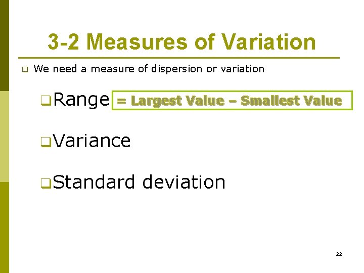
3 -2 Measures of Variation q We need a measure of dispersion or variation q. Range = Largest Value – Smallest Value q. Variance q. Standard deviation 22

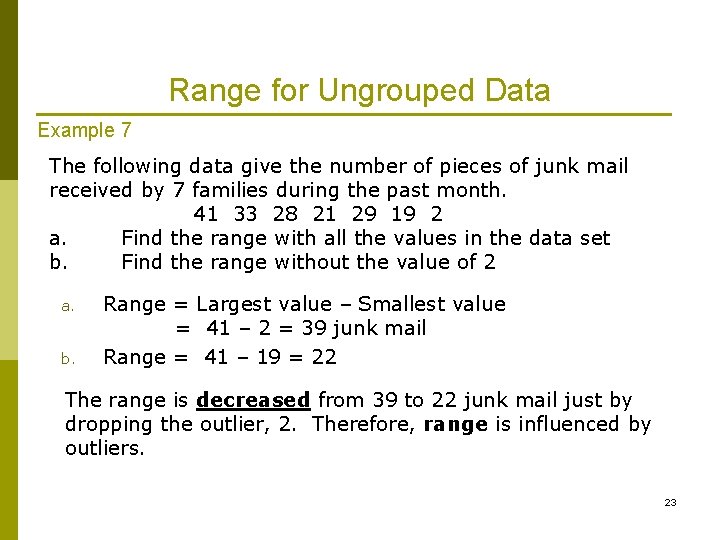
Range for Ungrouped Data Example 7 The following data give the number of pieces of junk mail received by 7 families during the past month. 41 33 28 21 29 19 2 a. Find the range with all the values in the data set b. Find the range without the value of 2 a. b. Range = Largest value – Smallest value = 41 – 2 = 39 junk mail Range = 41 – 19 = 22 The range is decreased from 39 to 22 junk mail just by dropping the outlier, 2. Therefore, range is influenced by outliers. 23

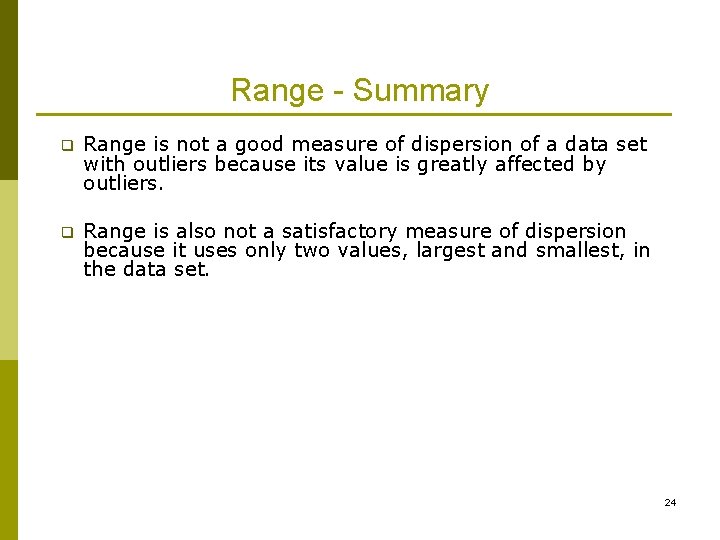
Range - Summary q Range is not a good measure of dispersion of a data set with outliers because its value is greatly affected by outliers. q Range is also not a satisfactory measure of dispersion because it uses only two values, largest and smallest, in the data set. 24

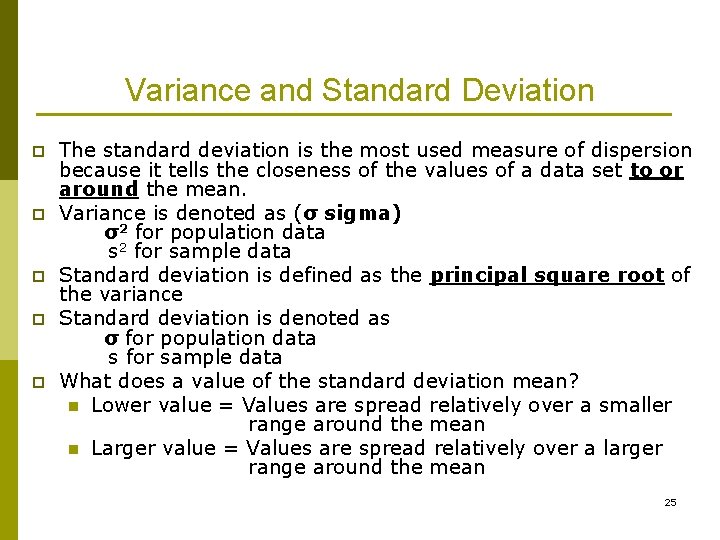
Variance and Standard Deviation p p p The standard deviation is the most used measure of dispersion because it tells the closeness of the values of a data set to or around the mean. Variance is denoted as (σ sigma) σ2 for population data s 2 for sample data Standard deviation is defined as the principal square root of the variance Standard deviation is denoted as σ for population data s for sample data What does a value of the standard deviation mean? n Lower value = Values are spread relatively over a smaller range around the mean n Larger value = Values are spread relatively over a larger range around the mean 25

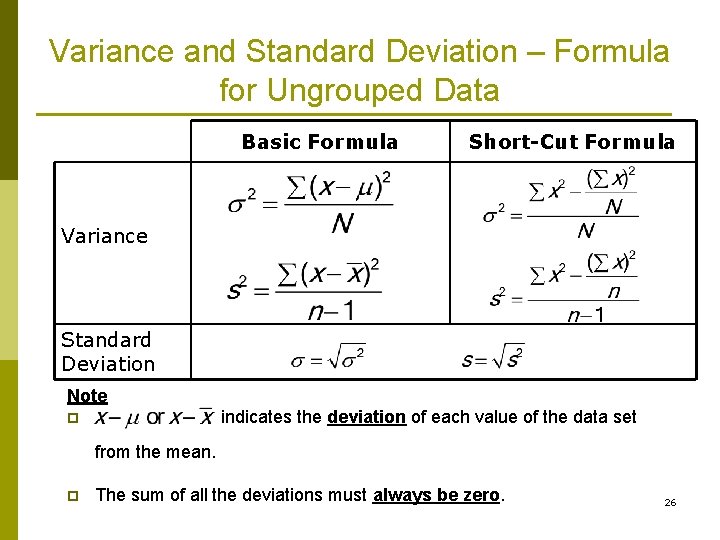
Variance and Standard Deviation – Formula for Ungrouped Data Basic Formula Short-Cut Formula Variance Standard Deviation Note p indicates the deviation of each value of the data set from the mean. p The sum of all the deviations must always be zero. 26

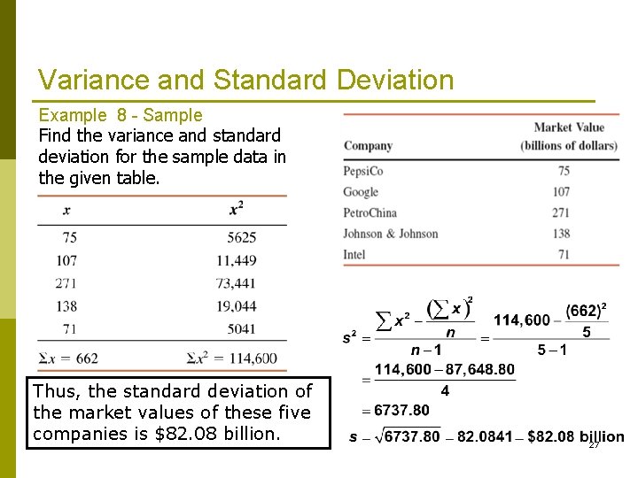
Variance and Standard Deviation Example 8 - Sample Find the variance and standard deviation for the sample data in the given table. Thus, the standard deviation of the market values of these five companies is $82. 08 billion. 27

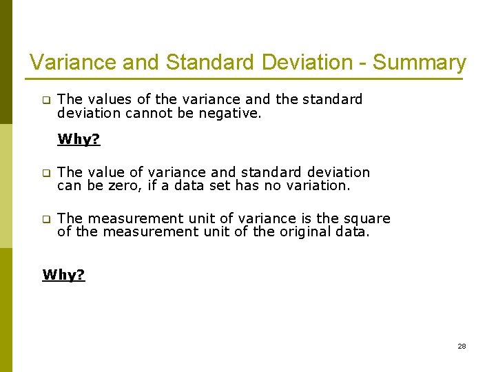
Variance and Standard Deviation - Summary q The values of the variance and the standard deviation cannot be negative. Why? q The value of variance and standard deviation can be zero, if a data set has no variation. q The measurement unit of variance is the square of the measurement unit of the original data. Why? 28

Population Parameters and Sample Statistics Mean, median, mode, range, variance, or standard deviation calculated for: n A population data set is called a population parameter or just parameter. µ and σ are examples of population parameters n A sample data set is called a sample statistic, or just statistic. are example of sample statistic. 29

USE OF STANDARD DEVIATION So far, we can find the mean and standard deviation of a distribution data. But the question is: q Whether we can use the mean and standard deviation to find the percentage or proportion of the data set that lie within an interval of the mean. q The answer is yes if we combine the mean and standard deviation. q To do this, we can use q Chebyshev’s theorem or q Empirical rule. q Our focus is only on the empirical rule 30

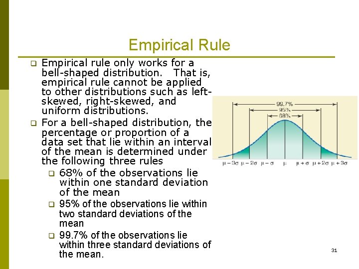
Empirical Rule q q Empirical rule only works for a bell-shaped distribution. That is, empirical rule cannot be applied to other distributions such as leftskewed, right-skewed, and uniform distributions. For a bell-shaped distribution, the percentage or proportion of a data set that lie within an interval of the mean is determined under the following three rules q 68% of the observations lie within one standard deviation of the mean q 95% of the observations lie within two standard deviations of the mean q 99. 7% of the observations lie within three standard deviations of the mean. 31

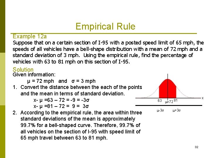
Empirical Rule Example 12 a Suppose that on a certain section of I-95 with a posted speed limit of 65 mph, the speeds of all vehicles have a bell-shape distribution with a mean of 72 mph and a standard deviation of 3 mph. Using the empirical rule, find the percentage of vehicles with 63 to 81 mph on this section of I-95. Solution Given information: µ = 72 mph and σ = 3 mph 1. Convert the distance between the each of the points and the mean in terms of standard deviation. x- µ =63 – 72 = -9 = -3σ x- µ =81 – 72 = 9 = 3σ 2. According to the empirical rule, the area within three standard deviations of the mean is approximately 99. 7% for a bell-shaped curve. Therefore, 99. 7% of all vehicles on the section of I-95 with speed limit of 65 mph travel between 63 to 81 mph. x 63 =72 81 -3 +3 32

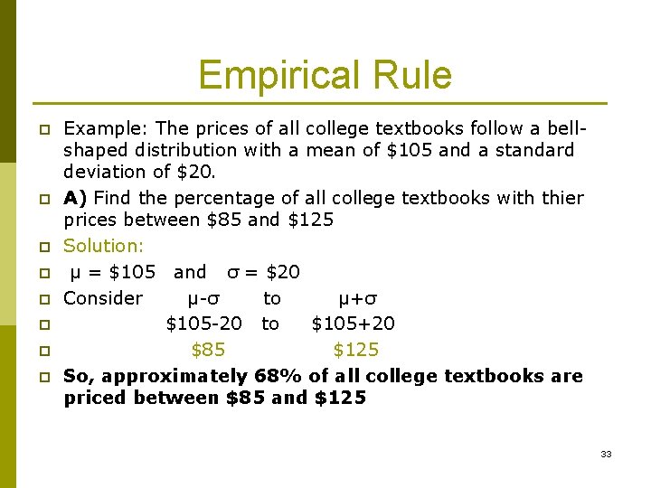
Empirical Rule p p p p Example: The prices of all college textbooks follow a bellshaped distribution with a mean of $105 and a standard deviation of $20. A) Find the percentage of all college textbooks with thier prices between $85 and $125 Solution: µ = $105 and σ = $20 Consider µ-σ to µ+σ $105 -20 to $105+20 $85 $125 So, approximately 68% of all college textbooks are priced between $85 and $125 33

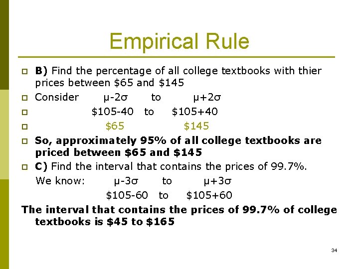
Empirical Rule B) Find the percentage of all college textbooks with thier prices between $65 and $145 p Consider µ-2σ to µ+2σ p $105 -40 to $105+40 p $65 $145 p So, approximately 95% of all college textbooks are priced between $65 and $145 p C) Find the interval that contains the prices of 99. 7%. We know: µ-3σ to µ+3σ $105 -60 to $105+60 The interval that contains the prices of 99. 7% of college textbooks is $45 to $165 p 34

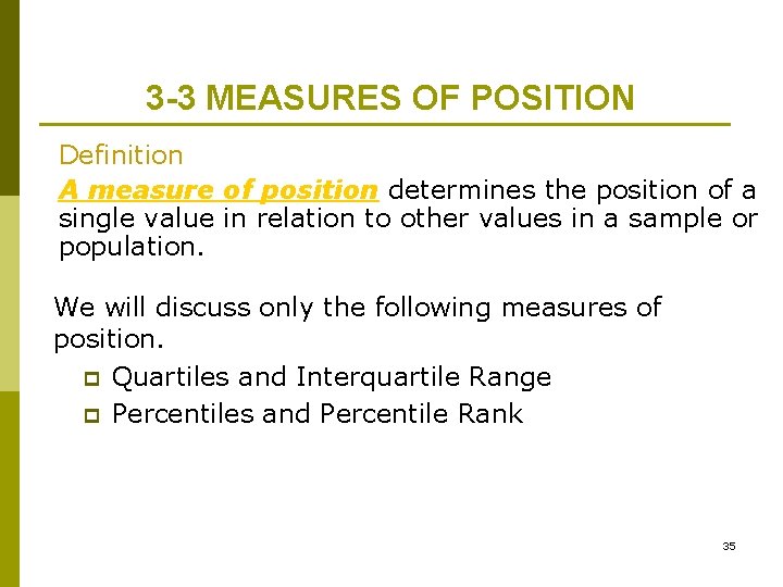
3 -3 MEASURES OF POSITION Definition A measure of position determines the position of a single value in relation to other values in a sample or population. We will discuss only the following measures of position. p Quartiles and Interquartile Range p Percentiles and Percentile Rank 35

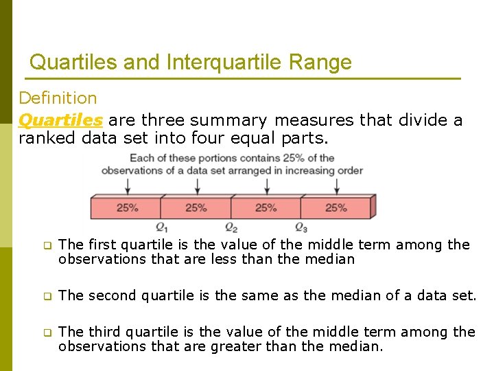
Quartiles and Interquartile Range Definition Quartiles are three summary measures that divide a ranked data set into four equal parts. q The first quartile is the value of the middle term among the observations that are less than the median q The second quartile is the same as the median of a data set. q The third quartile is the value of the middle term among the observations that are greater than the median.

Quartiles and Interquartile Range Calculating Interquartile Range Interquartile range is the difference between the third and first quartiles. That is, IQR = Interquartile range = Q 3 – Q 1

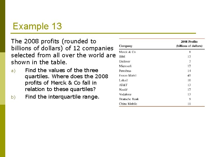
Example 13 The 2008 profits (rounded to billions of dollars) of 12 companies selected from all over the world are shown in the table. a) b) Find the values of the three quartiles. Where does the 2008 profits of Merck & Co fall in relation to these quartiles? Find the interquartile range.

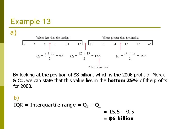
Example 13 a) By looking at the position of $8 billion, which is the 2008 profit of Merck & Co, we can state that this value lies in the bottom 25% of the profits for 2008. b) IQR = Interquartile range = Q 3 – Q 1 = 15. 5 – 9. 5 = $6 billion

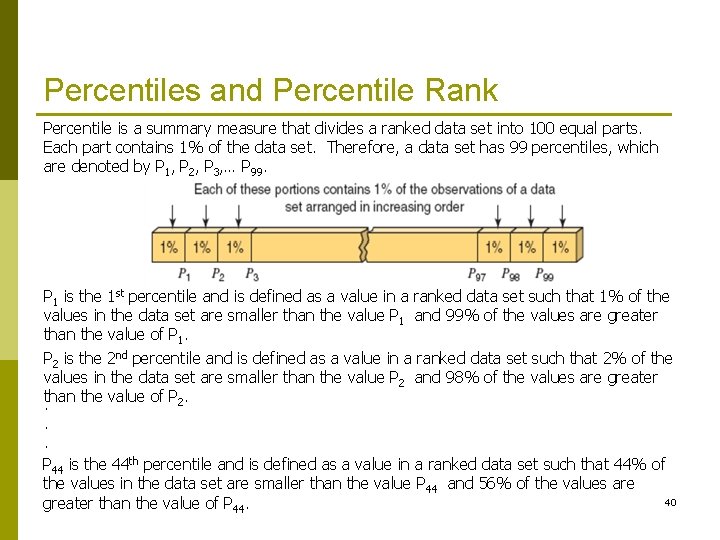
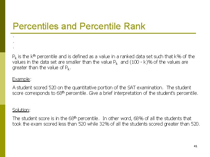
Percentiles and Percentile Rank Percentile is a summary measure that divides a ranked data set into 100 equal parts. Each part contains 1% of the data set. Therefore, a data set has 99 percentiles, which are denoted by P 1, P 2, P 3, … P 99. P 1 is the 1 st percentile and is defined as a value in a ranked data set such that 1% of the values in the data set are smaller than the value P 1 and 99% of the values are greater than the value of P 1. P 2 is the 2 nd percentile and is defined as a value in a ranked data set such that 2% of the values in the data set are smaller than the value P 2 and 98% of the values are greater. than the value of P 2. . . P 44 is the 44 th percentile and is defined as a value in a ranked data set such that 44% of the values in the data set are smaller than the value P 44 and 56% of the values are 40 greater than the value of P 44.

Percentiles and Percentile Rank. . . Pk is the kth percentile and is defined as a value in a ranked data set such that k% of the values in the data set are smaller than the value Pk and (100 - k)% of the values are greater than the value of Pk. Example: A student scored 520 on the quantitative portion of the SAT examination. The student score corresponds to 68 th percentile. Give a brief interpretation of the student's percentile. Solution: The student score is in the 68 th percentile. In other word, 68% of all the students that took the exam scored less than 520 while 32% of all the students scored greater than 520. 41

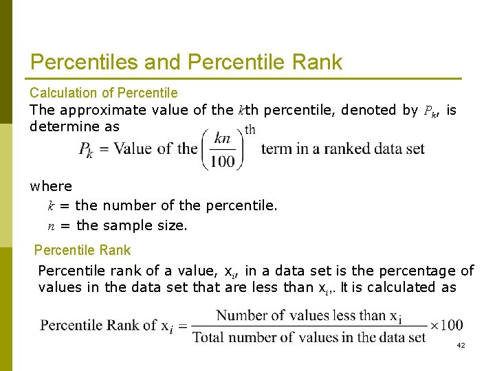
Percentiles and Percentile Rank Calculation of Percentile The approximate value of the kth percentile, denoted by Pk, is determine as where k = the number of the percentile. n = the sample size. Percentile Rank Percentile rank of a value, xi, in a data set is the percentage of values in the data set that are less than xi, . It is calculated as 42

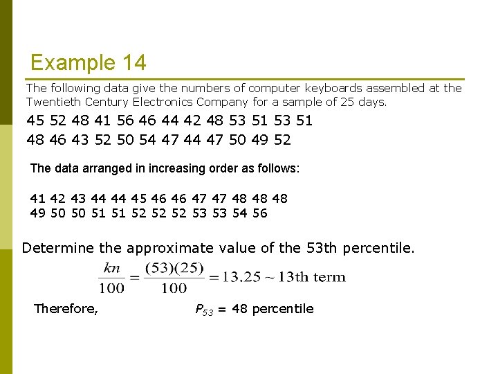
Example 14 The following data give the numbers of computer keyboards assembled at the Twentieth Century Electronics Company for a sample of 25 days. 45 52 48 41 56 46 44 42 48 53 51 48 46 43 52 50 54 47 44 47 50 49 52 The data arranged in increasing order as follows: 41 42 43 44 44 45 46 46 47 47 48 48 48 49 50 50 51 51 52 52 52 53 53 54 56 Determine the approximate value of the 53 th percentile. Therefore, P 53 = 48 percentile

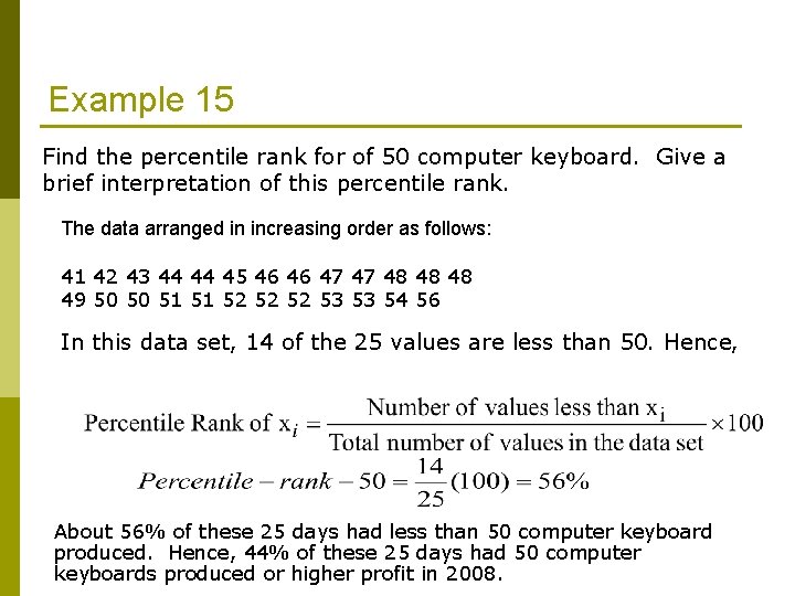
Example 15 Find the percentile rank for of 50 computer keyboard. Give a brief interpretation of this percentile rank. The data arranged in increasing order as follows: 41 42 43 44 44 45 46 46 47 47 48 48 48 49 50 50 51 51 52 52 52 53 53 54 56 In this data set, 14 of the 25 values are less than 50. Hence, About 56% of these 25 days had less than 50 computer keyboard produced. Hence, 44% of these 25 days had 50 computer keyboards produced or higher profit in 2008.

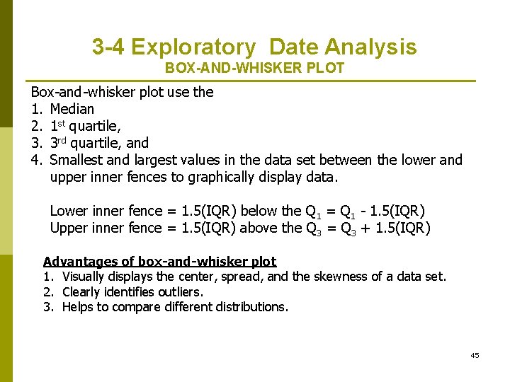
3 -4 Exploratory Date Analysis BOX-AND-WHISKER PLOT Box-and-whisker plot use the 1. Median 2. 1 st quartile, 3. 3 rd quartile, and 4. Smallest and largest values in the data set between the lower and upper inner fences to graphically display data. Lower inner fence = 1. 5(IQR) below the Q 1 = Q 1 - 1. 5(IQR) Upper inner fence = 1. 5(IQR) above the Q 3 = Q 3 + 1. 5(IQR) Advantages of box-and-whisker plot 1. Visually displays the center, spread, and the skewness of a data set. 2. Clearly identifies outliers. 3. Helps to compare different distributions. 45

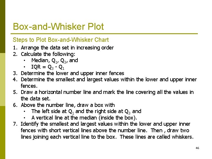
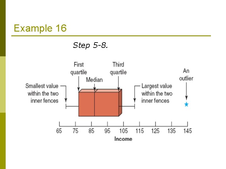
Box-and-Whisker Plot Steps to Plot Box-and-Whisker Chart 1. Arrange the data set in increasing order 2. Calculate the following: • Median, Q 1, Q 3, and • IQR = Q 3 - Q 1 3. Determine the lower and upper inner fences 4. Determine the smallest and largest values within the lower and upper inner fences. 5. Draw a horizontal number line and mark the line covering all the values in the data set. 6. Above the number line, draw a box with • The left side at Q 1 and the right side at Q 3 and • A vertical line at the median (inside the box). 7. Identify the smallest and largest values within the lower and upper inner fences with short vertical lines above the number line. Then , draw two lines joining each vertical line to the box. These lines are called whiskers. 46

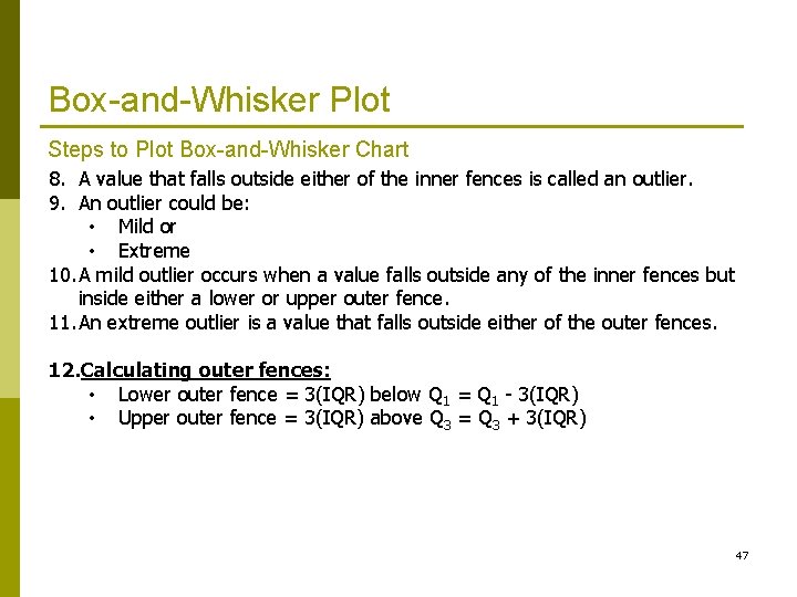
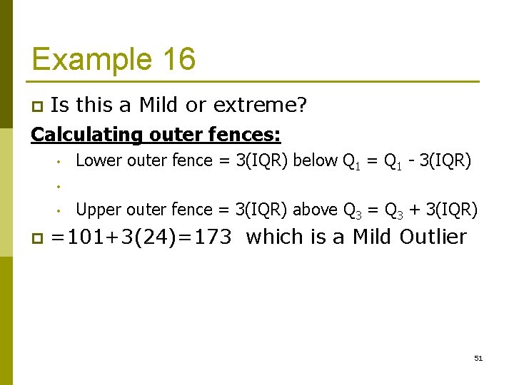
Box-and-Whisker Plot Steps to Plot Box-and-Whisker Chart 8. A value that falls outside either of the inner fences is called an outlier. 9. An outlier could be: • Mild or • Extreme 10. A mild outlier occurs when a value falls outside any of the inner fences but inside either a lower or upper outer fence. 11. An extreme outlier is a value that falls outside either of the outer fences. 12. Calculating outer fences: • Lower outer fence = 3(IQR) below Q 1 = Q 1 - 3(IQR) • Upper outer fence = 3(IQR) above Q 3 = Q 3 + 3(IQR) 47

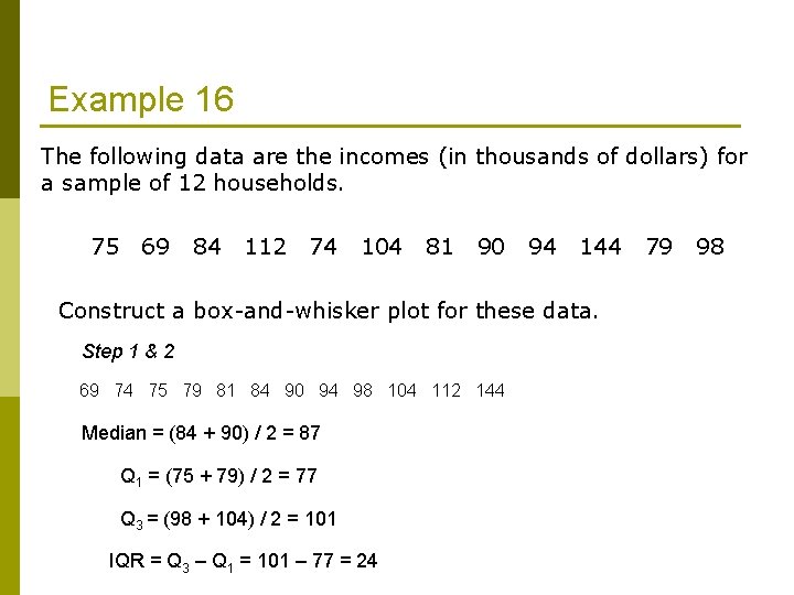
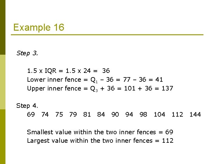
Example 16 The following data are the incomes (in thousands of dollars) for a sample of 12 households. 75 69 84 112 74 104 81 90 94 144 Construct a box-and-whisker plot for these data. Step 1 & 2 69 74 75 79 81 84 90 94 98 104 112 144 Median = (84 + 90) / 2 = 87 Q 1 = (75 + 79) / 2 = 77 Q 3 = (98 + 104) / 2 = 101 IQR = Q 3 – Q 1 = 101 – 77 = 24 79 98

Example 16 Step 3. 1. 5 x IQR = 1. 5 x 24 = 36 Lower inner fence = Q 1 – 36 = 77 – 36 = 41 Upper inner fence = Q 3 + 36 = 101 + 36 = 137 Step 4. 69 74 75 79 81 84 90 94 98 104 112 Smallest value within the two inner fences = 69 Largest value within the two inner fences = 112 144

Example 16 Step 5 -8.

Example 16 Is this a Mild or extreme? Calculating outer fences: p • Lower outer fence = 3(IQR) below Q 1 = Q 1 - 3(IQR) • • p Upper outer fence = 3(IQR) above Q 3 = Q 3 + 3(IQR) =101+3(24)=173 which is a Mild Outlier 51