Numerical Measures Numerical Measures Measures of Central Tendency

Numerical Measures

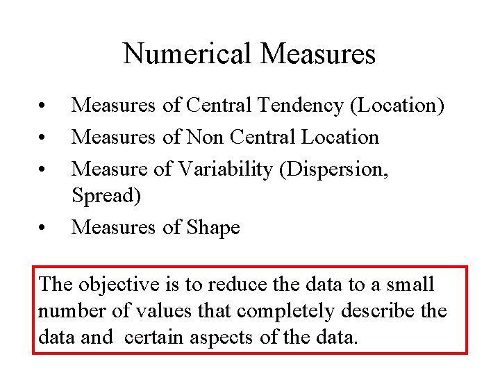
Numerical Measures • • Measures of Central Tendency (Location) Measures of Non Central Location Measure of Variability (Dispersion, Spread) Measures of Shape

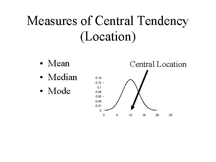
Measures of Central Tendency (Location) • Mean • Median • Mode Central Location

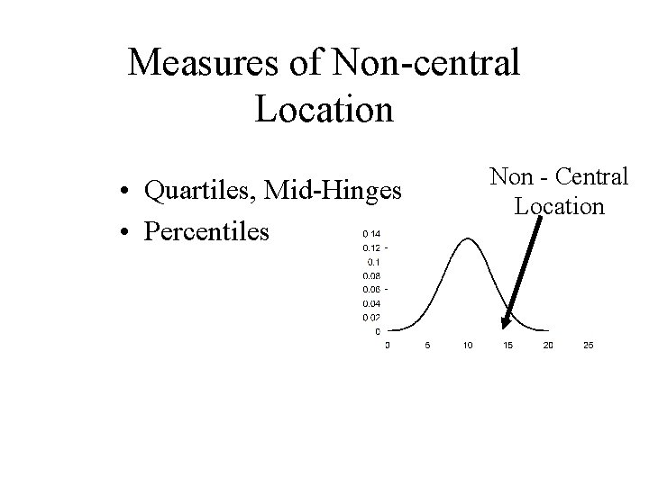
Measures of Non-central Location • Quartiles, Mid-Hinges • Percentiles Non - Central Location

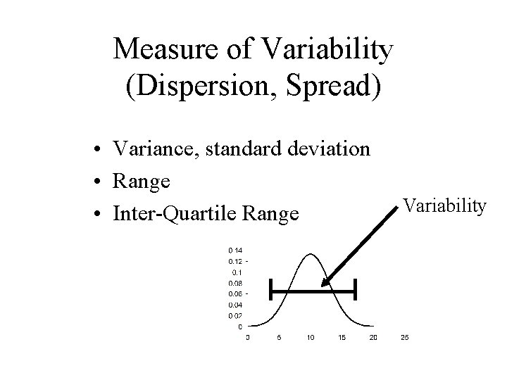
Measure of Variability (Dispersion, Spread) • Variance, standard deviation • Range • Inter-Quartile Range Variability

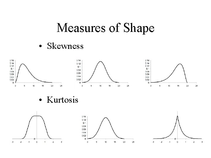
Measures of Shape • Skewness • Kurtosis

Summation Notation

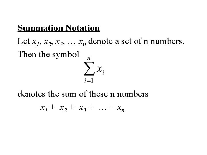
Summation Notation Let x 1, x 2, x 3, … xn denote a set of n numbers. Then the symbol denotes the sum of these n numbers x 1 + x 2 + x 3 + …+ xn

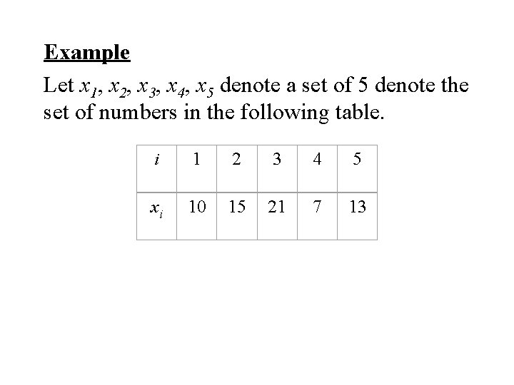
Example Let x 1, x 2, x 3, x 4, x 5 denote a set of 5 denote the set of numbers in the following table. i 1 2 3 4 5 xi 10 15 21 7 13

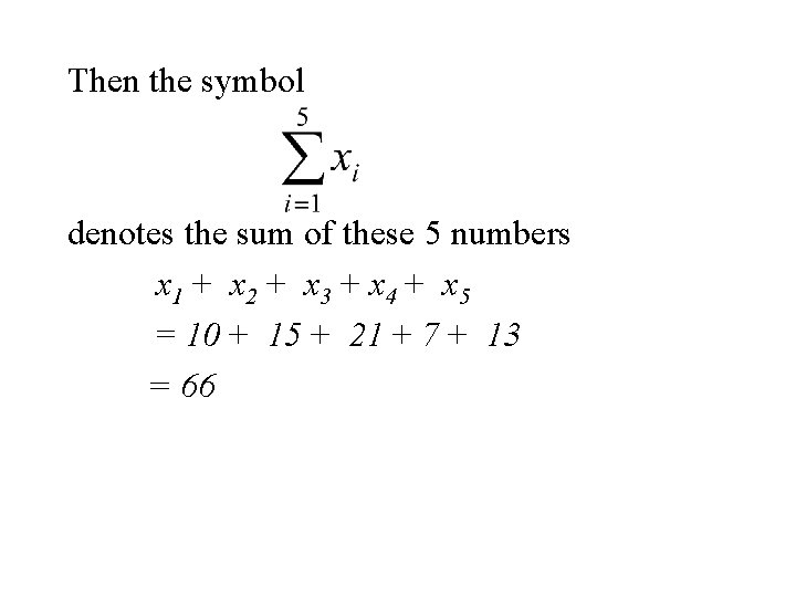
Then the symbol denotes the sum of these 5 numbers x 1 + x 2 + x 3 + x 4 + x 5 = 10 + 15 + 21 + 7 + 13 = 66

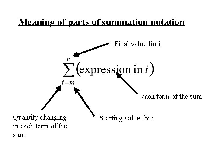
Meaning of parts of summation notation Final value for i each term of the sum Quantity changing in each term of the sum Starting value for i

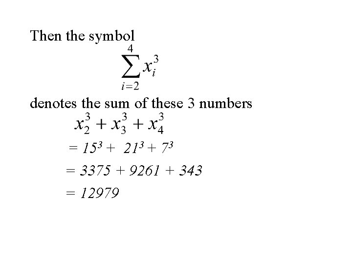
Example Again let x 1, x 2, x 3, x 4, x 5 denote a set of 5 denote the set of numbers in the following table. i 1 2 3 4 5 xi 10 15 21 7 13

Then the symbol denotes the sum of these 3 numbers = 153 + 213 + 73 = 3375 + 9261 + 343 = 12979

Measures of Central Location (Mean)

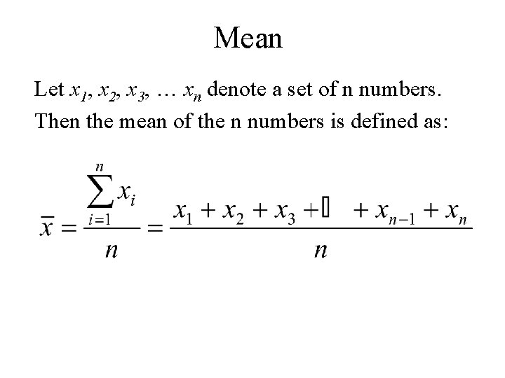
Mean Let x 1, x 2, x 3, … xn denote a set of n numbers. Then the mean of the n numbers is defined as:

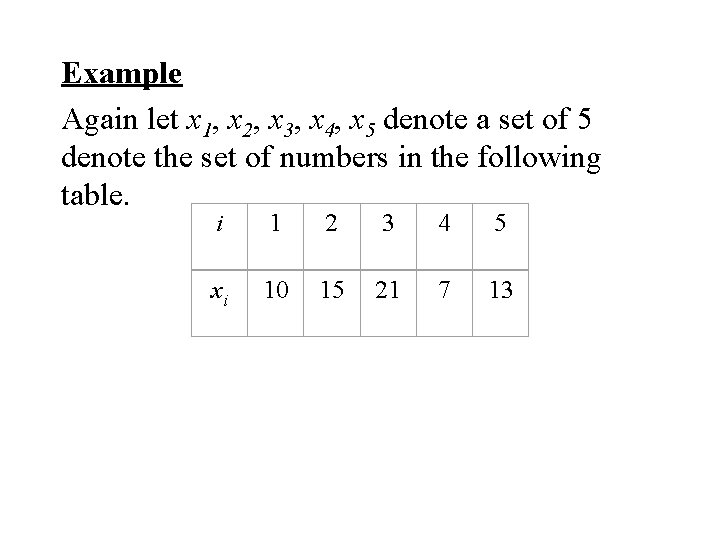
Example Again let x 1, x 2, x 3, x 4, x 5 denote a set of 5 denote the set of numbers in the following table. i 1 2 3 4 5 xi 10 15 21 7 13

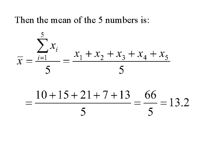
Then the mean of the 5 numbers is:

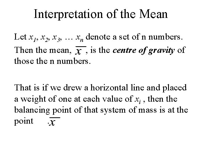
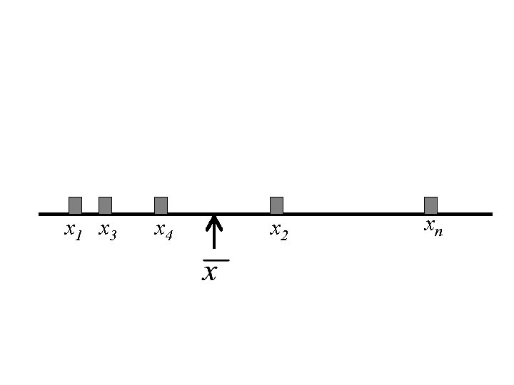
Interpretation of the Mean Let x 1, x 2, x 3, … xn denote a set of n numbers. Then the mean, , is the centre of gravity of those the n numbers. That is if we drew a horizontal line and placed a weight of one at each value of xi , then the balancing point of that system of mass is at the point .

x 1 x 3 x 4 x 2 xn

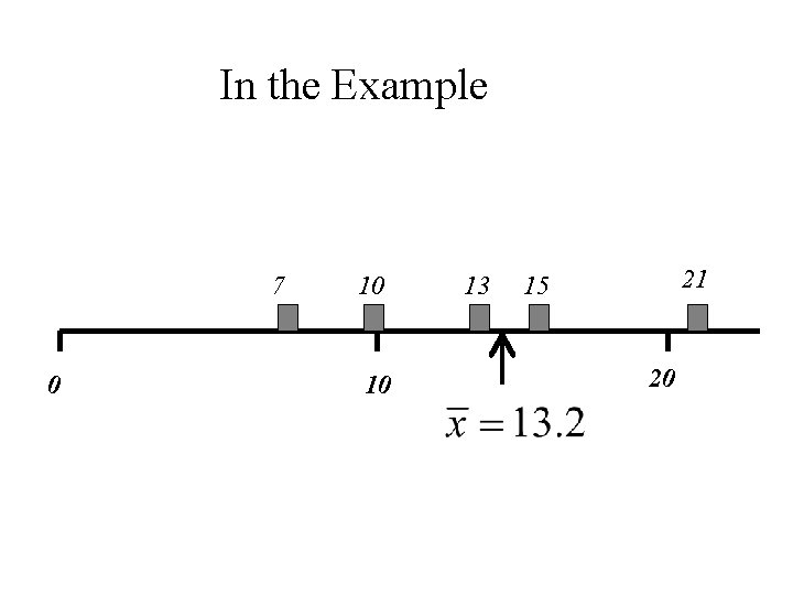
In the Example 7 0 10 10 13 21 15 20

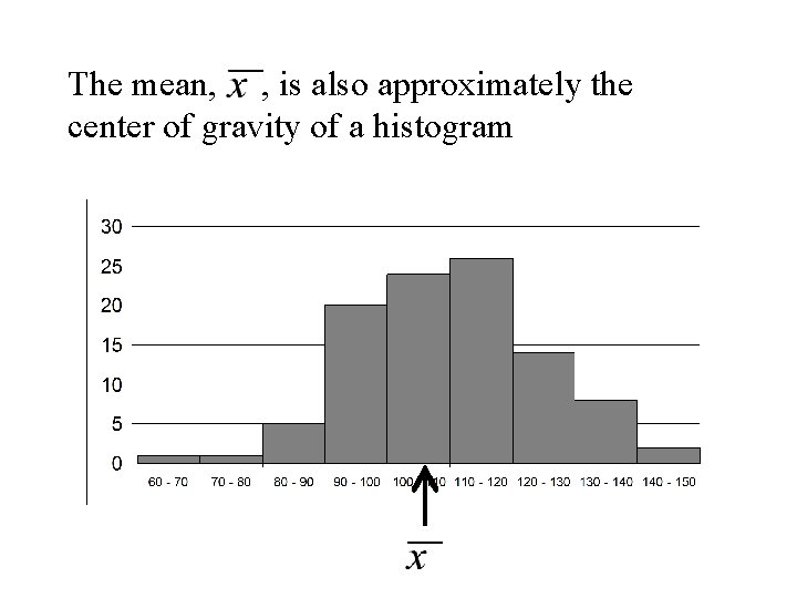
The mean, , is also approximately the center of gravity of a histogram

Measures of Central Location (Median)

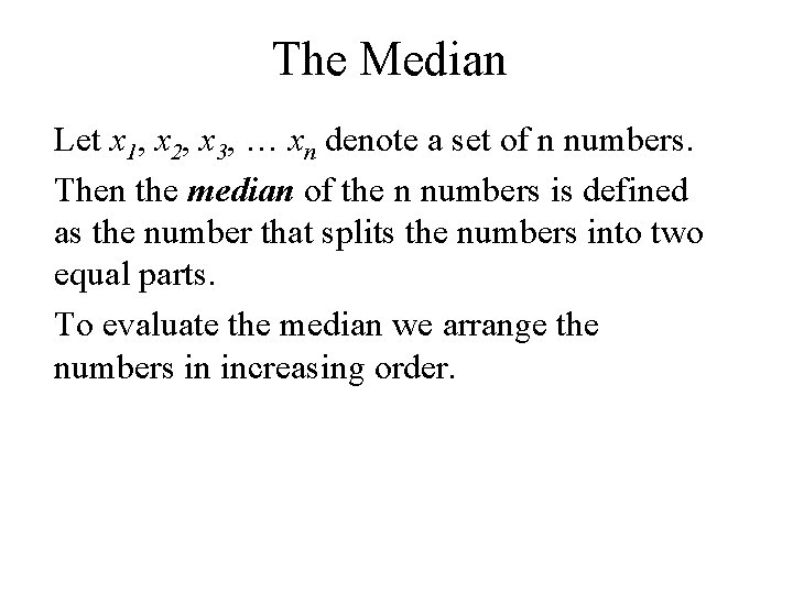
The Median Let x 1, x 2, x 3, … xn denote a set of n numbers. Then the median of the n numbers is defined as the number that splits the numbers into two equal parts. To evaluate the median we arrange the numbers in increasing order.

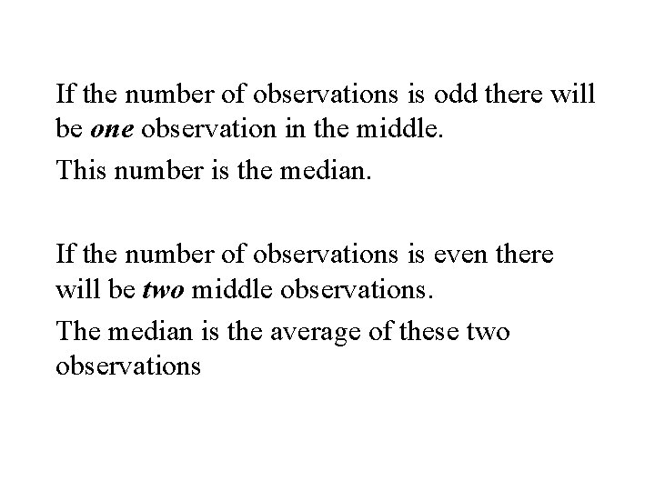
If the number of observations is odd there will be one observation in the middle. This number is the median. If the number of observations is even there will be two middle observations. The median is the average of these two observations

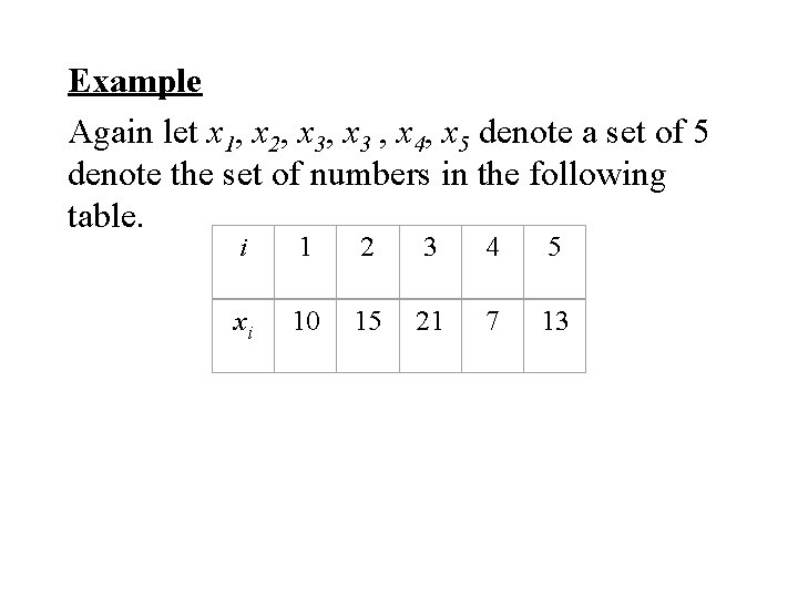
Example Again let x 1, x 2, x 3 , x 4, x 5 denote a set of 5 denote the set of numbers in the following table. i 1 2 3 4 5 xi 10 15 21 7 13

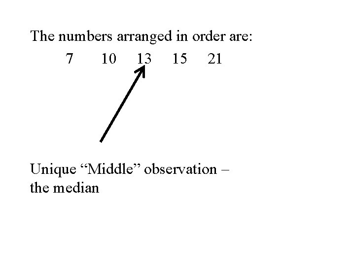
The numbers arranged in order are: 7 10 13 15 21 Unique “Middle” observation – the median

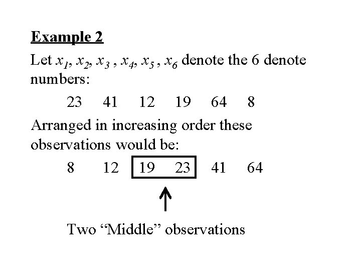
Example 2 Let x 1, x 2, x 3 , x 4, x 5 , x 6 denote the 6 denote numbers: 23 41 12 19 64 8 Arranged in increasing order these observations would be: 8 12 19 23 41 64 Two “Middle” observations

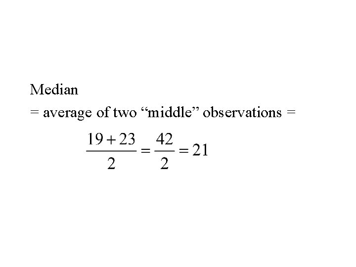
Median = average of two “middle” observations =

Example The data on N = 23 students Variables • Verbal IQ • Math IQ • Initial Reading Achievement Score • Final Reading Achievement Score

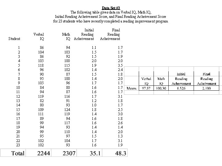
Student Verbal IQ 1 2 3 4 5 6 7 8 9 10 11 12 13 14 15 16 17 18 19 20 21 22 23 86 104 86 105 118 96 90 95 105 84 94 119 82 80 109 111 89 99 94 99 95 102 Data Set #3 The following table gives data on Verbal IQ, Math IQ, Initial Reading Acheivement Score, and Final Reading Acheivement Score for 23 students who have recently completed a reading improvement program Initial Final Math Reading IQ Acheivement 94 103 92 100 115 102 87 100 96 80 87 116 91 93 124 119 94 117 93 110 97 104 93 1. 1 1. 5 2. 0 1. 9 1. 4 1. 5 1. 4 1. 7 1. 6 1. 7 1. 2 1. 0 1. 8 1. 4 1. 6 1. 4 1. 5 1. 7 1. 6 1. 7 1. 9 2. 0 3. 5 2. 4 1. 8 2. 0 1. 7 3. 1 1. 8 1. 7 2. 5 3. 0 1. 8 2. 6 1. 4 2. 0 1. 3 3. 1 1. 9

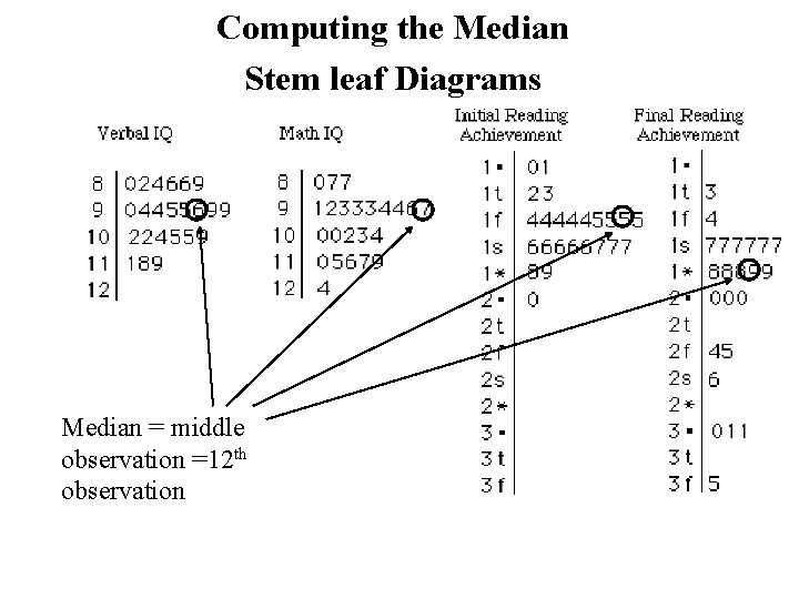
Computing the Median Stem leaf Diagrams Median = middle observation =12 th observation

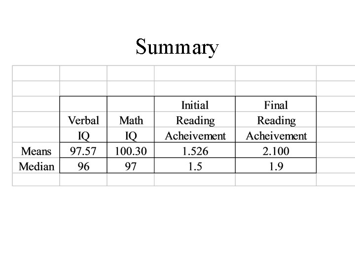
Summary

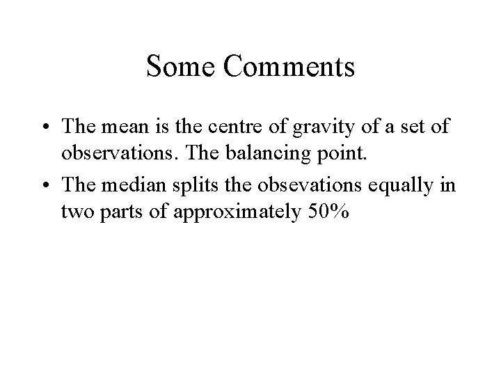
Some Comments • The mean is the centre of gravity of a set of observations. The balancing point. • The median splits the obsevations equally in two parts of approximately 50%

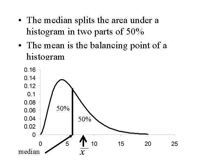
• The median splits the area under a histogram in two parts of 50% • The mean is the balancing point of a histogram 50% median

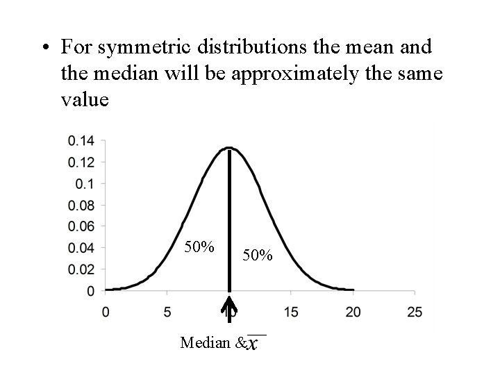
• For symmetric distributions the mean and the median will be approximately the same value 50% Median &

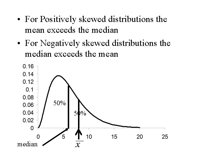
• For Positively skewed distributions the mean exceeds the median • For Negatively skewed distributions the median exceeds the mean 50% median

• An outlier is a “wild” observation in the data • Outliers occur because – of errors (typographical and computational) – Extreme cases in the population

• The mean is altered to a significant degree by the presence of outliers • Outliers have little effect on the value of the median • This is a reason for using the median in place of the mean as a measure of central location • Alternatively the mean is the best measure of central location when the data is Normally distributed (Bell-shaped)

Review

Summarizing Data Graphical Methods

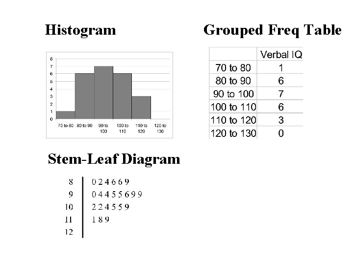
Histogram Stem-Leaf Diagram Grouped Freq Table

Numerical Measures • • Measures of Central Tendency (Location) Measures of Non Central Location Measure of Variability (Dispersion, Spread) Measures of Shape The objective is to reduce the data to a small number of values that completely describe the data and certain aspects of the data.

Measures of Central Location (Mean)

Mean Let x 1, x 2, x 3, … xn denote a set of n numbers. Then the mean of the n numbers is defined as:

Interpretation of the Mean Let x 1, x 2, x 3, … xn denote a set of n numbers. Then the mean, , is the centre of gravity of those the n numbers. That is if we drew a horizontal line and placed a weight of one at each value of xi , then the balancing point of that system of mass is at the point .

x 1 x 3 x 4 x 2 xn

The mean, , is also approximately the center of gravity of a histogram

The Median Let x 1, x 2, x 3, … xn denote a set of n numbers. Then the median of the n numbers is defined as the number that splits the numbers into two equal parts. To evaluate the median we arrange the numbers in increasing order.

If the number of observations is odd there will be one observation in the middle. This number is the median. If the number of observations is even there will be two middle observations. The median is the average of these two observations

Measures of Non-Central Location • • Percentiles Quartiles (Hinges, Mid-hinges)

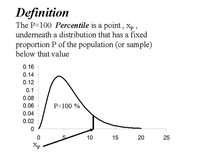
Definition The P× 100 Percentile is a point , x. P , underneath a distribution that has a fixed proportion P of the population (or sample) below that value P× 100 % x. P

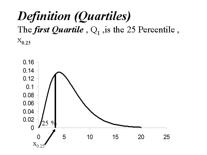
Definition (Quartiles) The first Quartile , Q 1 , is the 25 Percentile , x 0. 25 25 % x 0. 25

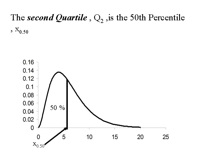
The second Quartile , Q 2 , is the 50 th Percentile , x 0. 50 50 % x 0. 50

• The second Quartile , Q 2 , is also the median and the 50 th percentile

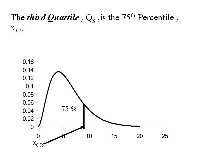
The third Quartile , Q 3 , is the 75 th Percentile , x 0. 75 75 % x 0. 75

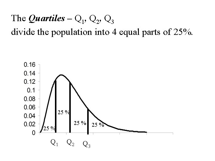
The Quartiles – Q 1, Q 2, Q 3 divide the population into 4 equal parts of 25%. 25 % Q 1 25 % Q 2 Q 3

Computing Percentiles and Quartiles • There are several methods used to compute percentiles and quartiles. Different computer packages will use different methods • Sometimes for small samples these methods will agree (but not always) • For large samples the methods will agree within a certain level of accuracy

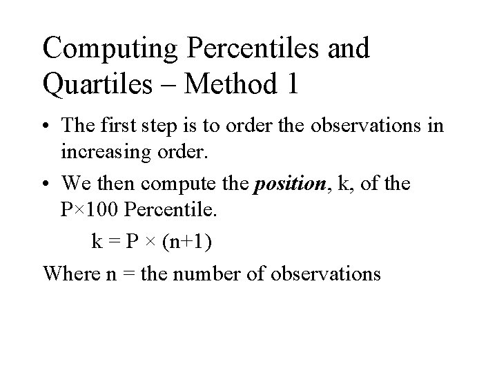
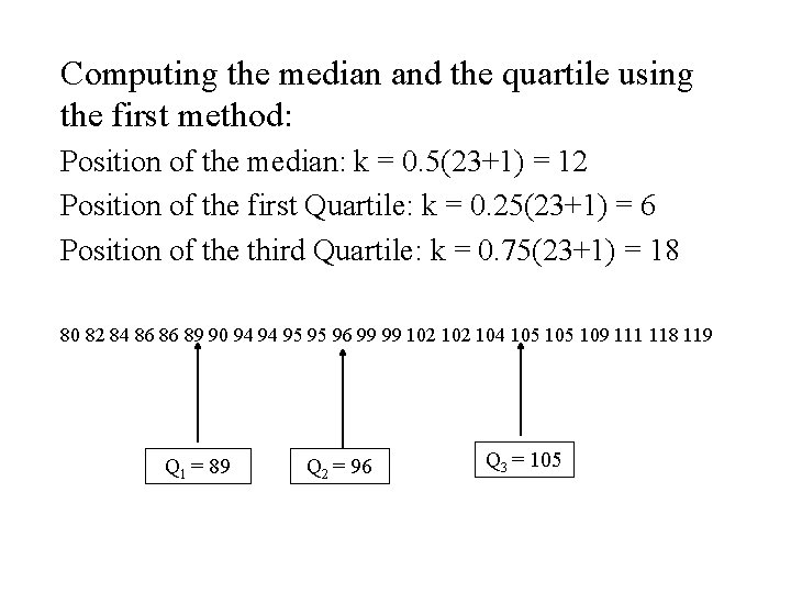
Computing Percentiles and Quartiles – Method 1 • The first step is to order the observations in increasing order. • We then compute the position, k, of the P× 100 Percentile. k = P × (n+1) Where n = the number of observations

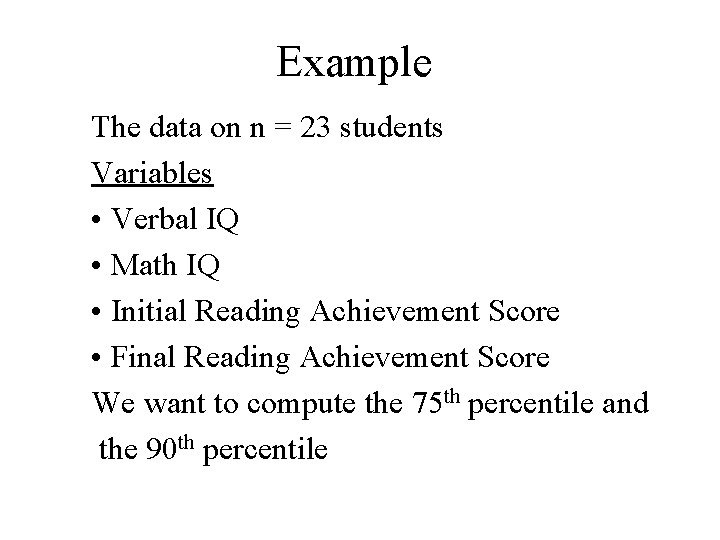
Example The data on n = 23 students Variables • Verbal IQ • Math IQ • Initial Reading Achievement Score • Final Reading Achievement Score We want to compute the 75 th percentile and the 90 th percentile

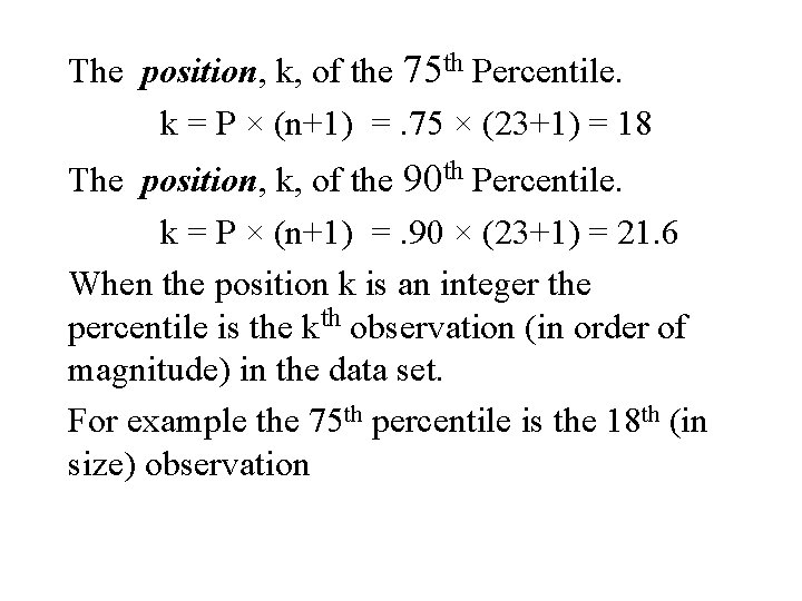
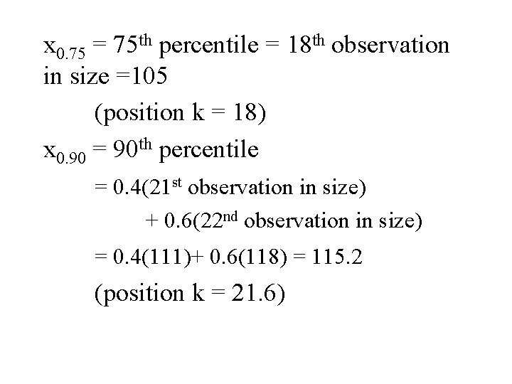
The position, k, of the 75 th Percentile. k = P × (n+1) =. 75 × (23+1) = 18 The position, k, of the 90 th Percentile. k = P × (n+1) =. 90 × (23+1) = 21. 6 When the position k is an integer the percentile is the kth observation (in order of magnitude) in the data set. For example the 75 th percentile is the 18 th (in size) observation

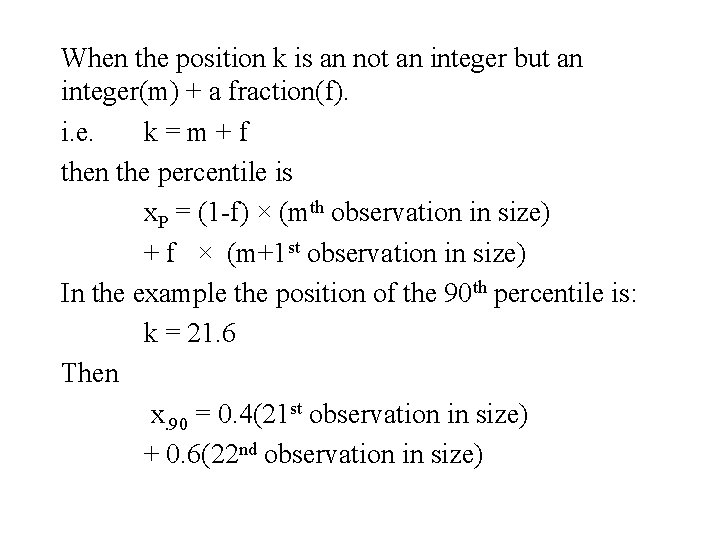
When the position k is an not an integer but an integer(m) + a fraction(f). i. e. k = m + f then the percentile is x. P = (1 -f) × (mth observation in size) + f × (m+1 st observation in size) In the example the position of the 90 th percentile is: k = 21. 6 Then x. 90 = 0. 4(21 st observation in size) + 0. 6(22 nd observation in size)

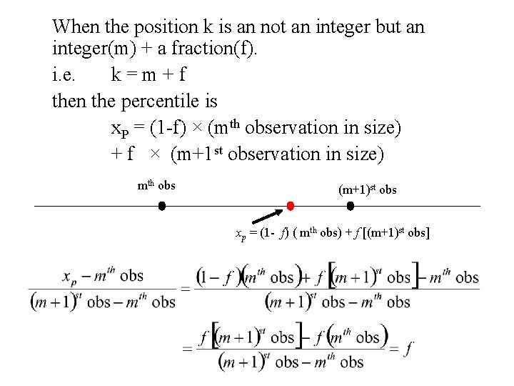
When the position k is an not an integer but an integer(m) + a fraction(f). i. e. k = m + f then the percentile is x. P = (1 -f) × (mth observation in size) + f × (m+1 st observation in size) mth obs (m+1)st obs xp = (1 - f) ( mth obs) + f [(m+1)st obs]

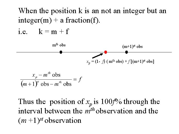
When the position k is an not an integer but an integer(m) + a fraction(f). i. e. k = m + f mth obs (m+1)st obs xp = (1 - f) ( mth obs) + f [(m+1)st obs] Thus the position of xp is 100 f% through the interval between the mth observation and the (m +1)st observation

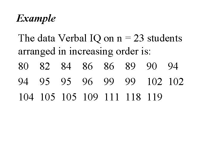
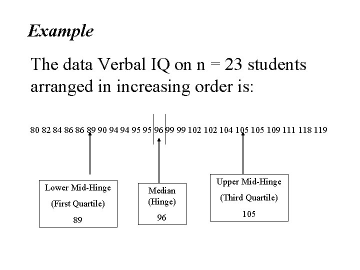
Example The data Verbal IQ on n = 23 students arranged in increasing order is: 80 82 84 86 86 89 90 94 94 95 95 96 99 99 102 104 105 109 111 118 119

x 0. 75 = 75 th percentile = 18 th observation in size =105 (position k = 18) x 0. 90 = 90 th percentile = 0. 4(21 st observation in size) + 0. 6(22 nd observation in size) = 0. 4(111)+ 0. 6(118) = 115. 2 (position k = 21. 6)

An Alternative method for computing Quartiles – Method 2 • Sometimes this method will result in the same values for the quartiles. • Sometimes this method will result in the different values for the quartiles. • For large samples the two methods will result in approximately the same answer.

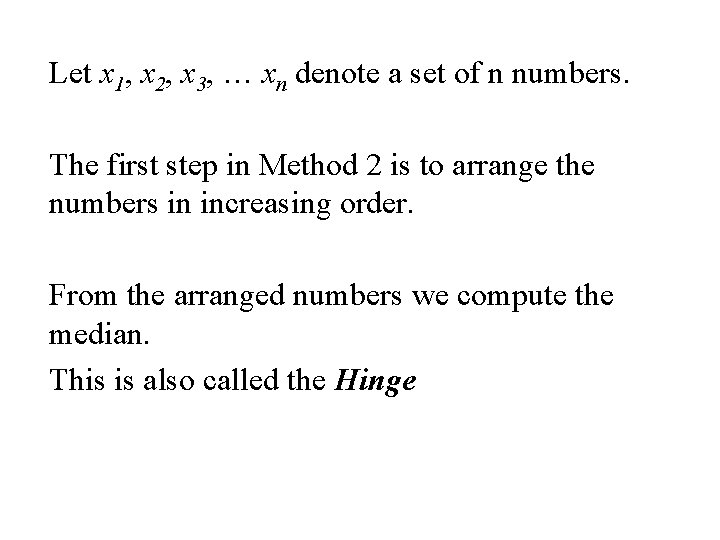
Let x 1, x 2, x 3, … xn denote a set of n numbers. The first step in Method 2 is to arrange the numbers in increasing order. From the arranged numbers we compute the median. This is also called the Hinge

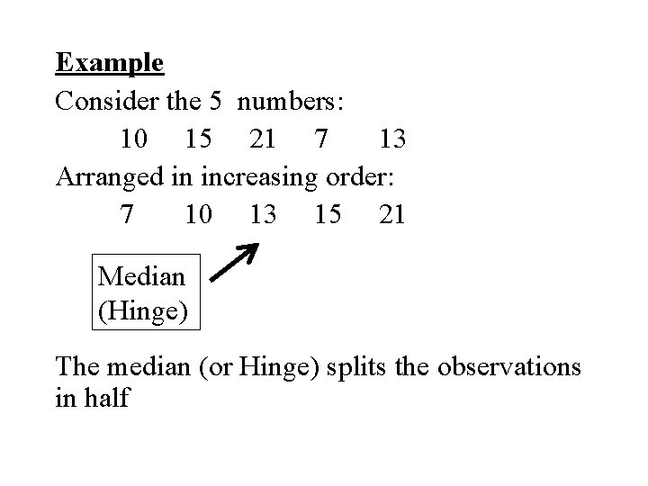
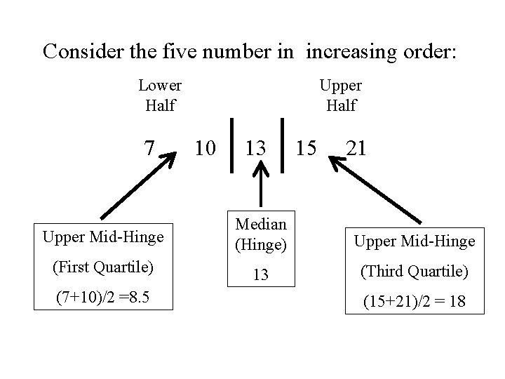
Example Consider the 5 numbers: 10 15 21 7 13 Arranged in increasing order: 7 10 13 15 21 Median (Hinge) The median (or Hinge) splits the observations in half

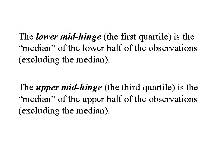
The lower mid-hinge (the first quartile) is the “median” of the lower half of the observations (excluding the median). The upper mid-hinge (the third quartile) is the “median” of the upper half of the observations (excluding the median).

Consider the five number in increasing order: Lower Upper Half 7 Half 10 13 15 21 Upper Mid-Hinge Median (Hinge) Upper Mid-Hinge (First Quartile) 13 (Third Quartile) (7+10)/2 =8. 5 (15+21)/2 = 18

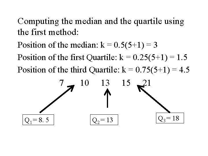
Computing the median and the quartile using the first method: Position of the median: k = 0. 5(5+1) = 3 Position of the first Quartile: k = 0. 25(5+1) = 1. 5 Position of the third Quartile: k = 0. 75(5+1) = 4. 5 7 Q 1 = 8. 5 10 13 Q 2 = 13 15 21 Q 3 = 18

• Both methods result in the same value • This is not always true.

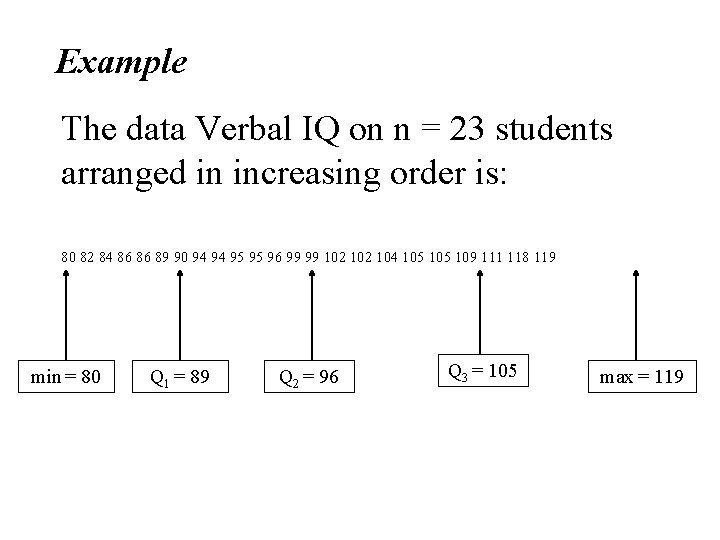
Example The data Verbal IQ on n = 23 students arranged in increasing order is: 80 82 84 86 86 89 90 94 94 95 95 96 99 99 102 104 105 109 111 118 119 Lower Mid-Hinge (First Quartile) Median (Hinge) 89 96 Upper Mid-Hinge (Third Quartile) 105

Computing the median and the quartile using the first method: Position of the median: k = 0. 5(23+1) = 12 Position of the first Quartile: k = 0. 25(23+1) = 6 Position of the third Quartile: k = 0. 75(23+1) = 18 80 82 84 86 86 89 90 94 94 95 95 96 99 99 102 104 105 109 111 118 119 Q 1 = 89 Q 2 = 96 Q 3 = 105

• Many programs compute percentiles, quartiles etc. • Each may use different methods. • It is important to know which method is being used. • The different methods result in answers that are close when the sample size is large.

Announcement Assignment 2 has been posted this assignment has to be handed in and is due Friday, January 22 This assignment requires the use of a Statistical Package (SPSS or Minitab) available in most computer labs. Instructions on the use of these packages will be given in the lab today

Box-Plots Box-Whisker Plots • A graphical method of displaying data • An alternative to the histogram and stem-leaf diagram

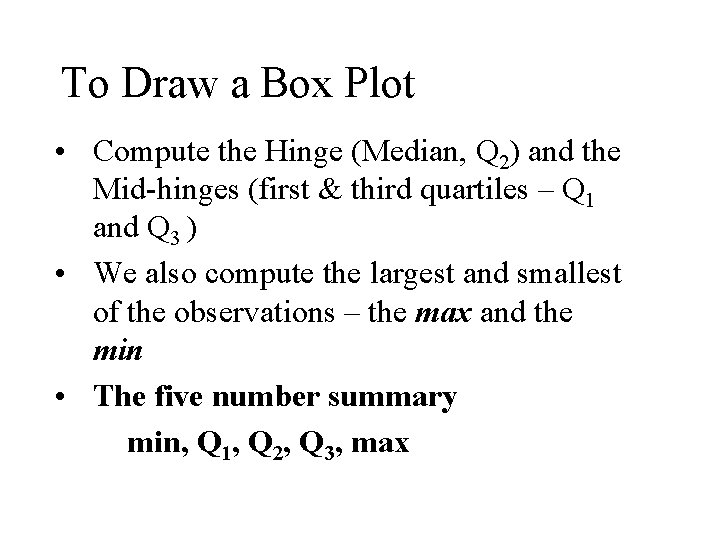
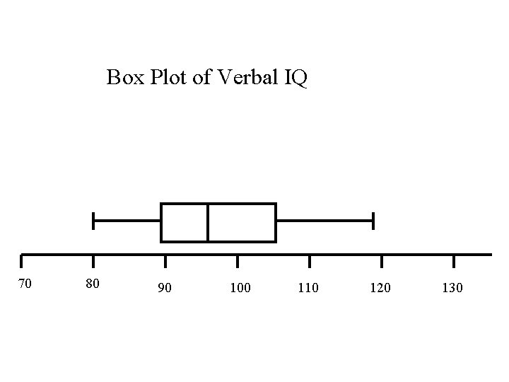
To Draw a Box Plot • Compute the Hinge (Median, Q 2) and the Mid-hinges (first & third quartiles – Q 1 and Q 3 ) • We also compute the largest and smallest of the observations – the max and the min • The five number summary min, Q 1, Q 2, Q 3, max

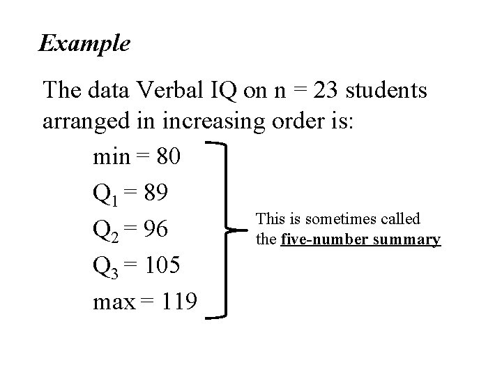
Example The data Verbal IQ on n = 23 students arranged in increasing order is: 80 82 84 86 86 89 90 94 94 95 95 96 99 99 102 104 105 109 111 118 119 min = 80 Q 1 = 89 Q 2 = 96 Q 3 = 105 max = 119

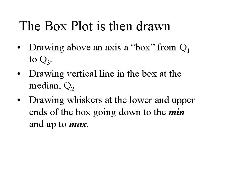
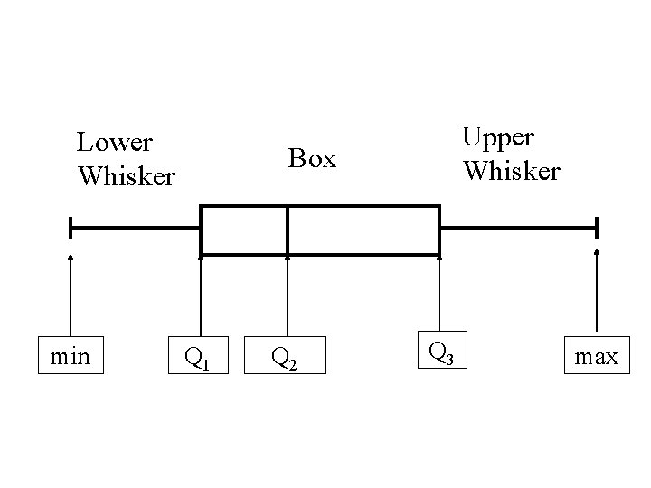
The Box Plot is then drawn • Drawing above an axis a “box” from Q 1 to Q 3. • Drawing vertical line in the box at the median, Q 2 • Drawing whiskers at the lower and upper ends of the box going down to the min and up to max.

Lower Whisker min Upper Whisker Box Q 1 Q 2 Q 3 max

Example The data Verbal IQ on n = 23 students arranged in increasing order is: min = 80 Q 1 = 89 This is sometimes called Q 2 = 96 the five-number summary Q 3 = 105 max = 119

Box Plot of Verbal IQ 70 80 90 100 110 120 130

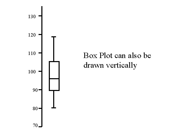
130 120 110 100 90 80 70 Box Plot can also be drawn vertically

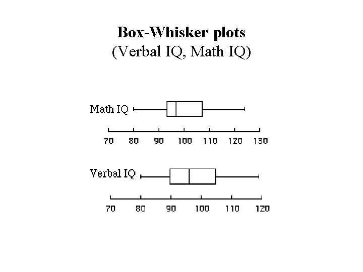
Box-Whisker plots (Verbal IQ, Math IQ)

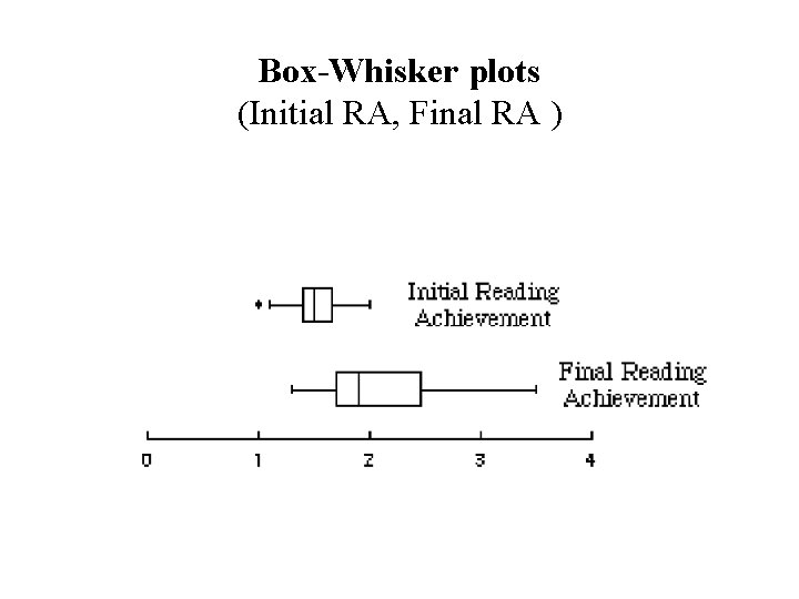
Box-Whisker plots (Initial RA, Final RA )

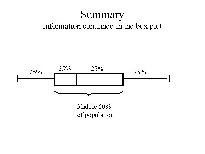
Summary Information contained in the box plot 25% 25% Middle 50% of population 25%

Advance Box Plots

• An outlier is a “wild” observation in the data • Outliers occur because – of errors (typographical and computational) – Extreme cases in the population • We will now consider the drawing of boxplots where outliers are identified

To Draw a Box Plot we need to: • Compute the Hinge (Median, Q 2) and the Mid-hinges (first & third quartiles – Q 1 and Q 3 ) • The difference Q 3– Q 1 is called the interquartile range (denoted by IQR) • To identify outliers we will compute the inner and outer fences

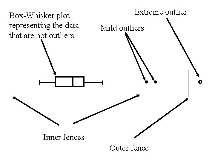
The fences are like the fences at a prison. We expect the entire population to be within both sets of fences. If a member of the population is between the inner and outer fences it is a mild outlier. If a member of the population is outside of the outer fences it is an extreme outlier.

Inner fences

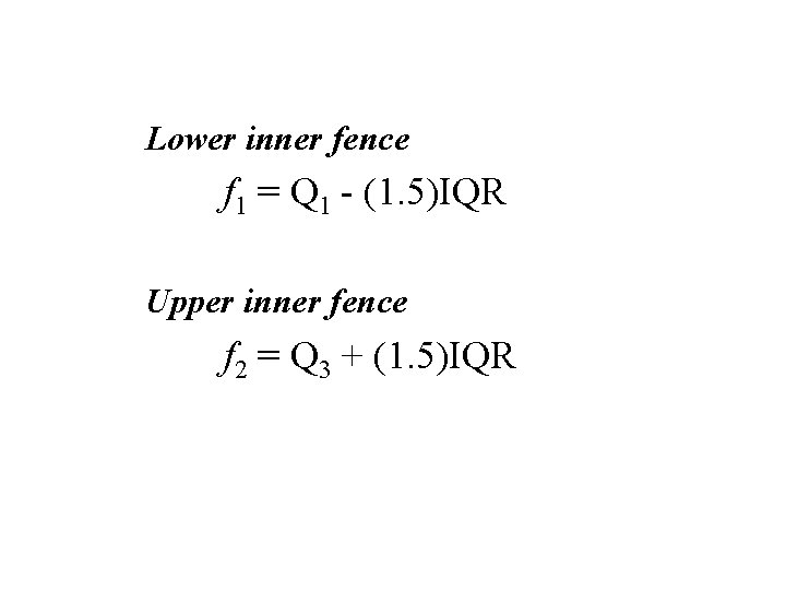
Lower inner fence f 1 = Q 1 - (1. 5)IQR Upper inner fence f 2 = Q 3 + (1. 5)IQR

Outer fences

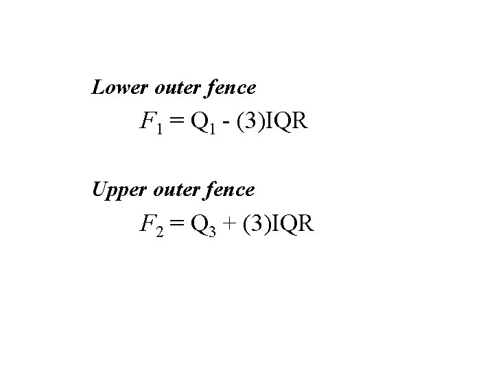
Lower outer fence F 1 = Q 1 - (3)IQR Upper outer fence F 2 = Q 3 + (3)IQR

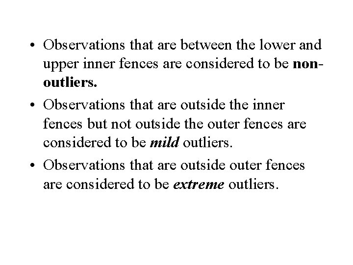
• Observations that are between the lower and upper inner fences are considered to be nonoutliers. • Observations that are outside the inner fences but not outside the outer fences are considered to be mild outliers. • Observations that are outside outer fences are considered to be extreme outliers.

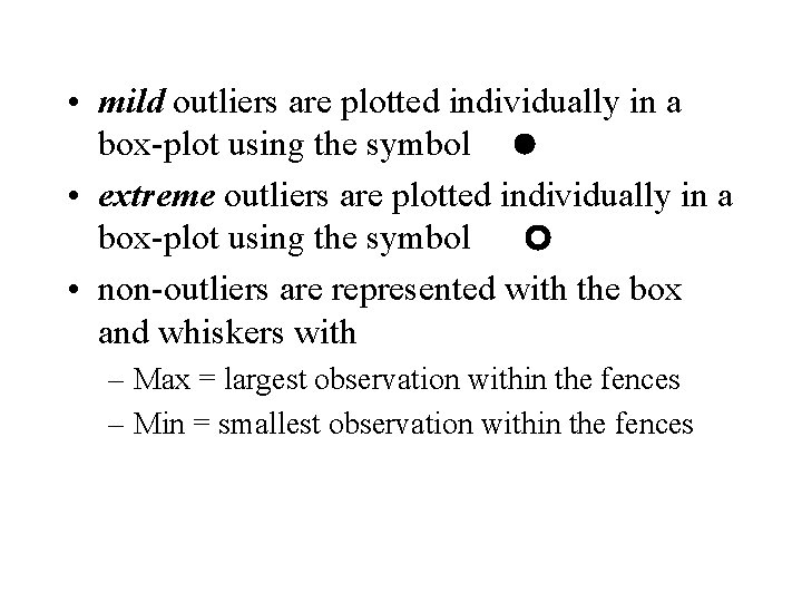
• mild outliers are plotted individually in a box-plot using the symbol • extreme outliers are plotted individually in a box-plot using the symbol • non-outliers are represented with the box and whiskers with – Max = largest observation within the fences – Min = smallest observation within the fences

Box-Whisker plot representing the data that are not outliers Extreme outlier Mild outliers Inner fences Outer fence

Example Data collected on n = 109 countries in 1995. Data collected on k = 25 variables.

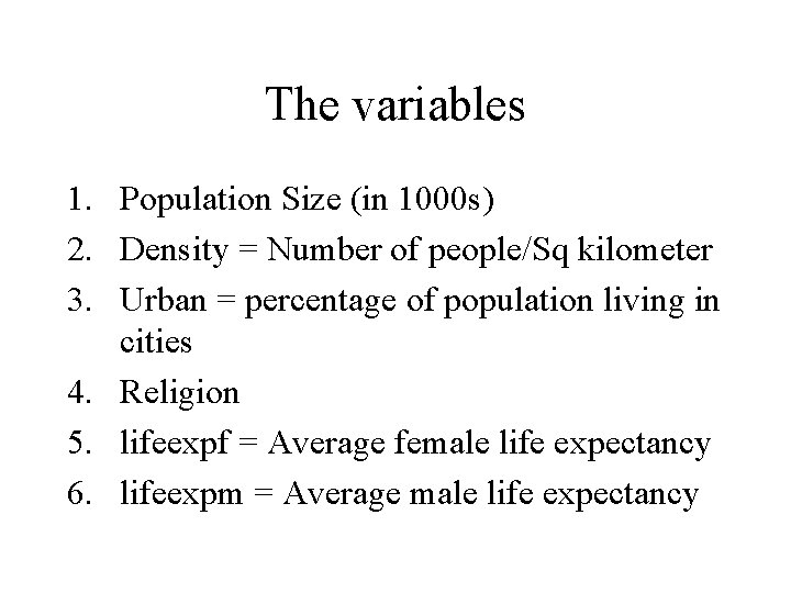
The variables 1. Population Size (in 1000 s) 2. Density = Number of people/Sq kilometer 3. Urban = percentage of population living in cities 4. Religion 5. lifeexpf = Average female life expectancy 6. lifeexpm = Average male life expectancy

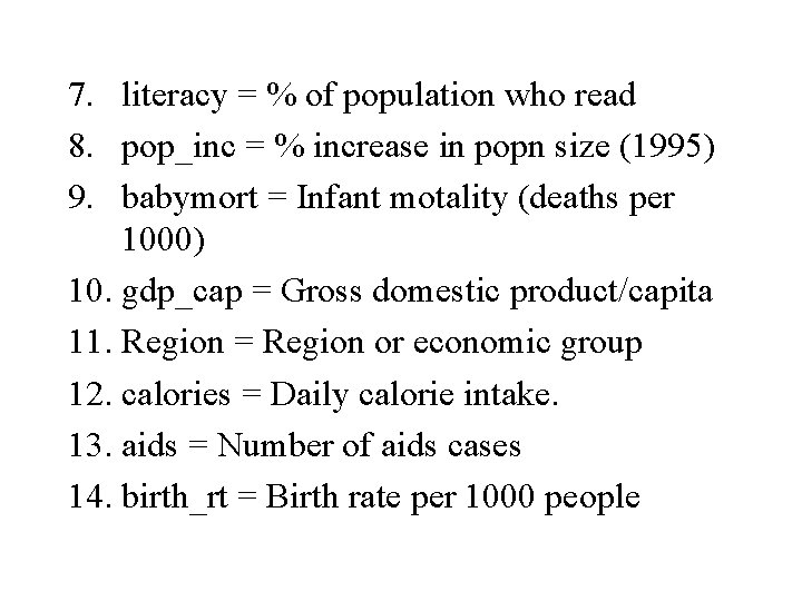
7. literacy = % of population who read 8. pop_inc = % increase in popn size (1995) 9. babymort = Infant motality (deaths per 1000) 10. gdp_cap = Gross domestic product/capita 11. Region = Region or economic group 12. calories = Daily calorie intake. 13. aids = Number of aids cases 14. birth_rt = Birth rate per 1000 people

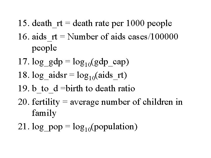
15. death_rt = death rate per 1000 people 16. aids_rt = Number of aids cases/100000 people 17. log_gdp = log 10(gdp_cap) 18. log_aidsr = log 10(aids_rt) 19. b_to_d =birth to death ratio 20. fertility = average number of children in family 21. log_pop = log 10(population)

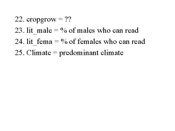
22. cropgrow = ? ? 23. lit_male = % of males who can read 24. lit_fema = % of females who can read 25. Climate = predominant climate

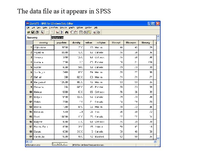
The data file as it appears in SPSS

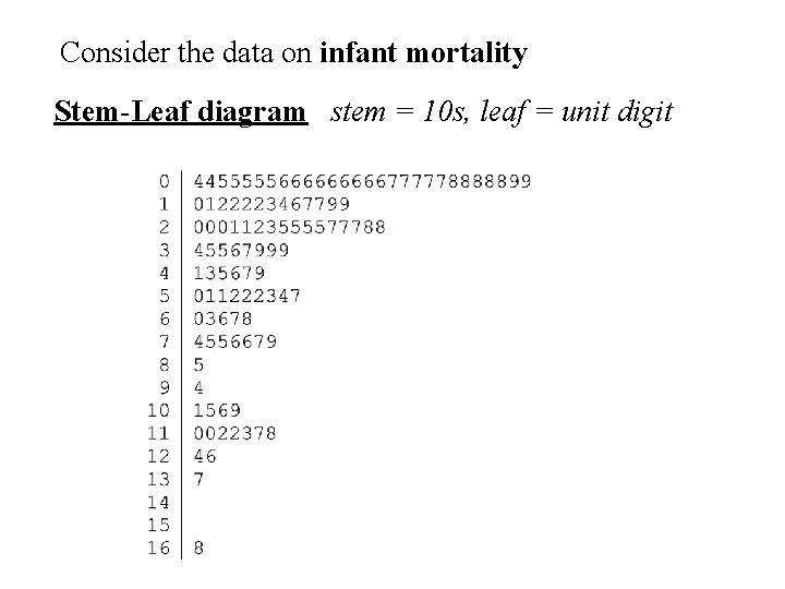
Consider the data on infant mortality Stem-Leaf diagram stem = 10 s, leaf = unit digit

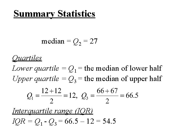
Summary Statistics median = Q 2 = 27 Quartiles Lower quartile = Q 1 = the median of lower half Upper quartile = Q 3 = the median of upper half Interquartile range (IQR) IQR = Q 1 - Q 3 = 66. 5 – 12 = 54. 5

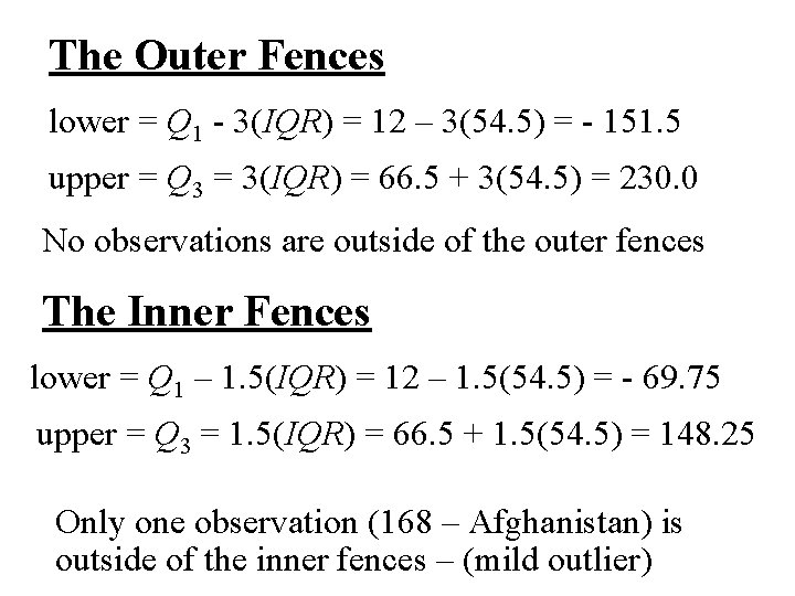
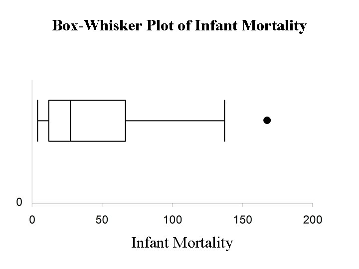
The Outer Fences lower = Q 1 - 3(IQR) = 12 – 3(54. 5) = - 151. 5 upper = Q 3 = 3(IQR) = 66. 5 + 3(54. 5) = 230. 0 No observations are outside of the outer fences The Inner Fences lower = Q 1 – 1. 5(IQR) = 12 – 1. 5(54. 5) = - 69. 75 upper = Q 3 = 1. 5(IQR) = 66. 5 + 1. 5(54. 5) = 148. 25 Only one observation (168 – Afghanistan) is outside of the inner fences – (mild outlier)

Box-Whisker Plot of Infant Mortality

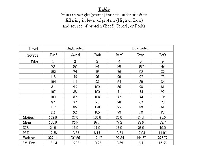
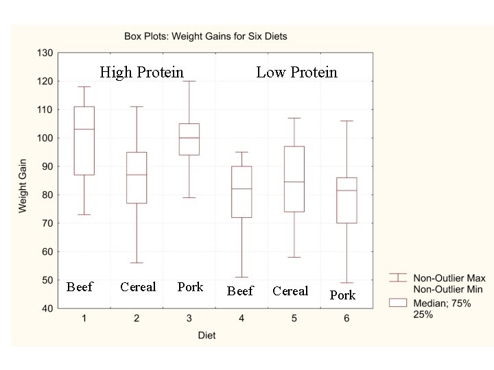
Example 2 In this example we are looking at the weight gains (grams) for rats under six diets differing in level of protein (High or Low) and source of protein (Beef, Cereal, or Pork). – Ten test animals for each diet

Table Gains in weight (grams) for rats under six diets differing in level of protein (High or Low) and source of protein (Beef, Cereal, or Pork) High Protein Level Source Diet Median Mean IQR PSD Variance Std. Dev. Low protein Beef Cereal Pork Beef Cereal Pork 1 73 102 118 104 81 107 100 87 111 103. 0 100. 0 24. 0 17. 78 229. 11 15. 14 2 98 74 56 111 95 88 82 77 86 92 87. 0 85. 9 18. 0 13. 33 225. 66 15. 02 3 94 79 96 98 102 108 91 120 105 100. 0 99. 5 11. 0 8. 15 119. 17 10. 92 4 90 76 90 64 86 51 72 90 95 78 82. 0 79. 2 18. 0 13. 33 192. 84 13. 89 5 107 95 97 80 98 74 74 67 89 58 84. 5 83. 9 23. 0 17. 04 246. 77 15. 71 6 49 82 73 86 81 97 106 70 61 82 81. 5 78. 7 16. 0 11. 05 273. 79 16. 55

High Protein Beef Cereal Pork Low Protein Beef Cereal Pork

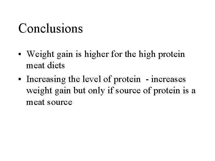
Conclusions • Weight gain is higher for the high protein meat diets • Increasing the level of protein - increases weight gain but only if source of protein is a meat source

Next topic: Numerical Measures of Variability