Numerical Measures Numerical Measures Measures of Central Tendency

Numerical Measures

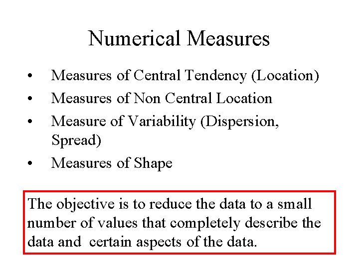
Numerical Measures • • Measures of Central Tendency (Location) Measures of Non Central Location Measure of Variability (Dispersion, Spread) Measures of Shape

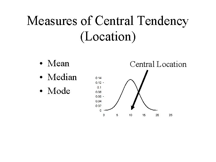
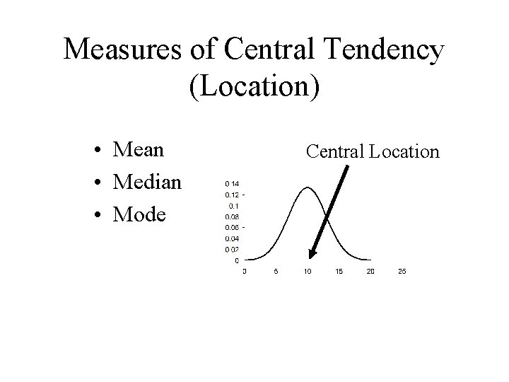
Measures of Central Tendency (Location) • Mean • Median • Mode Central Location

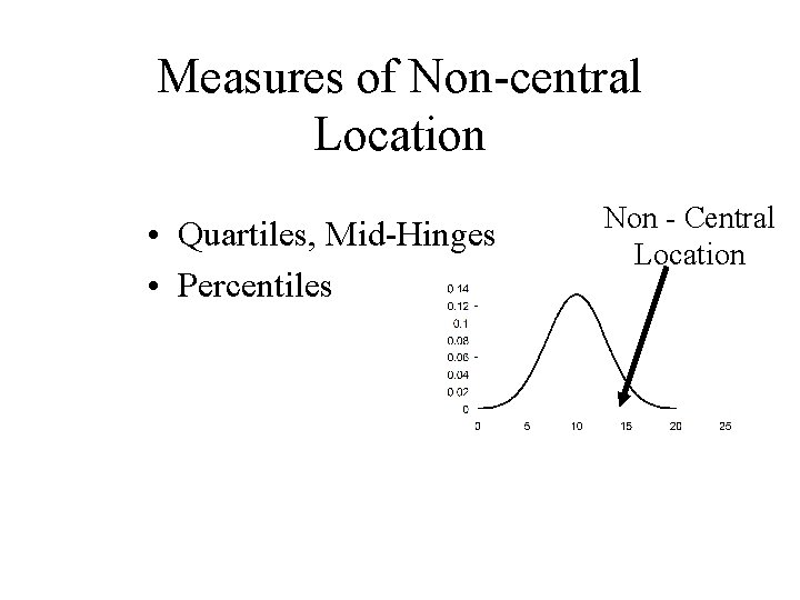
Measures of Non-central Location • Quartiles, Mid-Hinges • Percentiles Non - Central Location

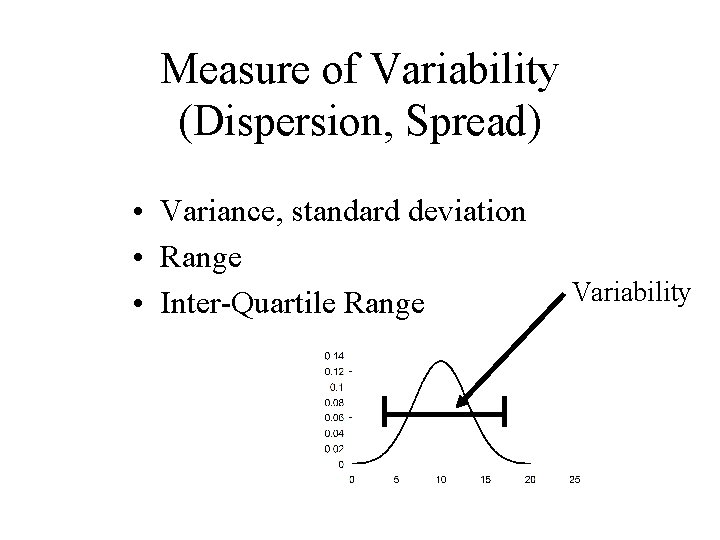
Measure of Variability (Dispersion, Spread) • Variance, standard deviation • Range • Inter-Quartile Range Variability

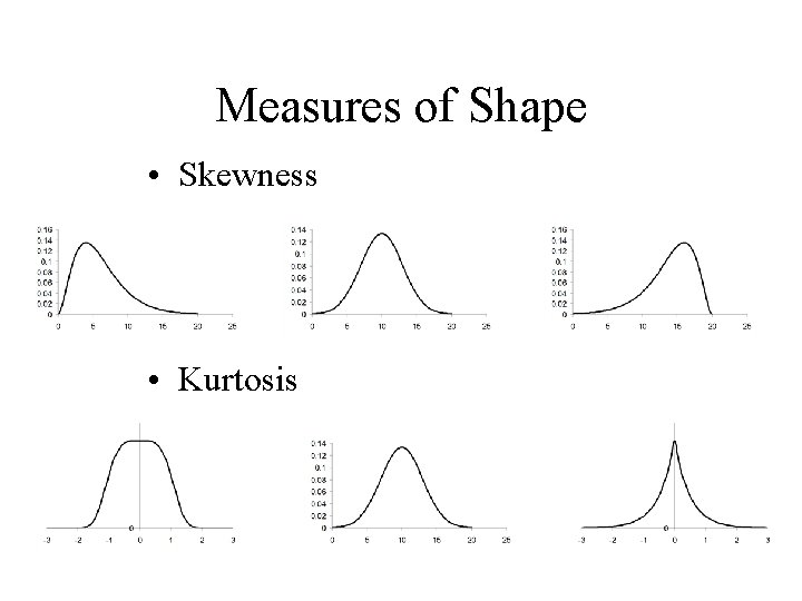
Measures of Shape • Skewness • Kurtosis

Summation Notation

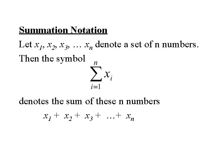
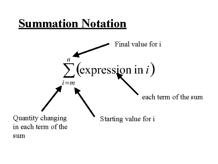
Summation Notation Let x 1, x 2, x 3, … xn denote a set of n numbers. Then the symbol denotes the sum of these n numbers x 1 + x 2 + x 3 + …+ xn

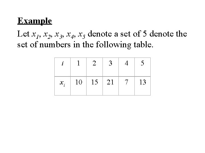
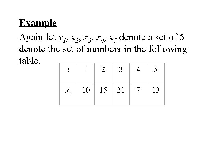
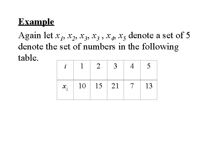
Example Let x 1, x 2, x 3, x 4, x 5 denote a set of 5 denote the set of numbers in the following table. i 1 2 3 4 5 xi 10 15 21 7 13

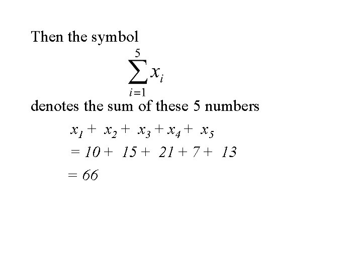
Then the symbol denotes the sum of these 5 numbers x 1 + x 2 + x 3 + x 4 + x 5 = 10 + 15 + 21 + 7 + 13 = 66

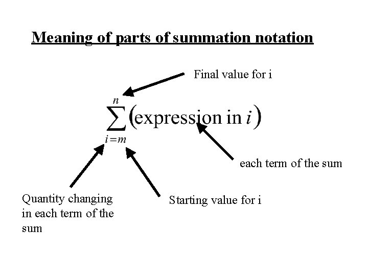
Meaning of parts of summation notation Final value for i each term of the sum Quantity changing in each term of the sum Starting value for i

Example Again let x 1, x 2, x 3, x 4, x 5 denote a set of 5 denote the set of numbers in the following table. i 1 2 3 4 5 xi 10 15 21 7 13

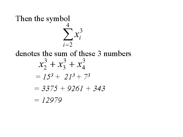
Then the symbol denotes the sum of these 3 numbers = 153 + 213 + 73 = 3375 + 9261 + 343 = 12979

Measures of Central Location (Mean)

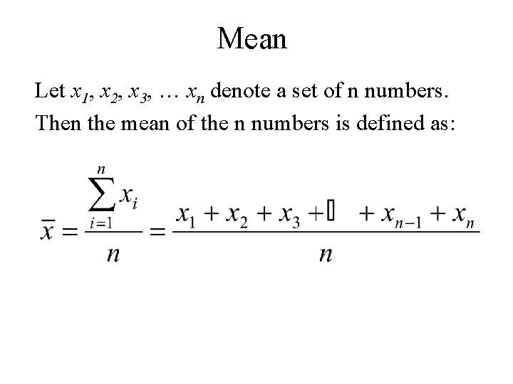
Mean Let x 1, x 2, x 3, … xn denote a set of n numbers. Then the mean of the n numbers is defined as:

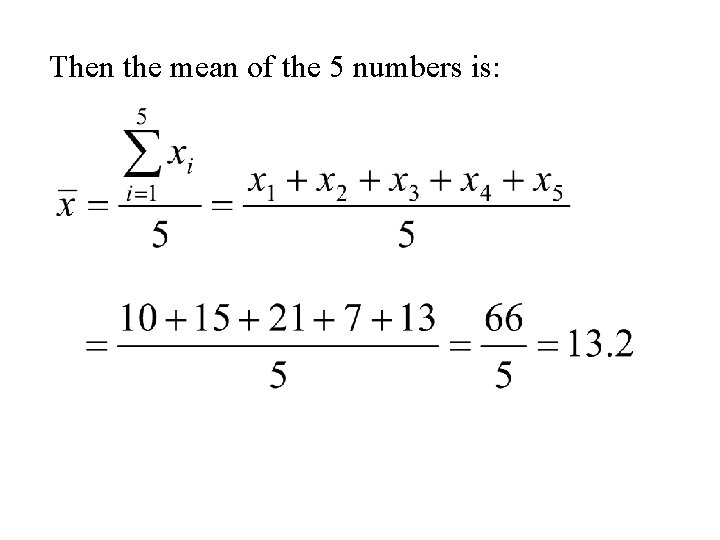
Example Again let x 1, x 2, x 3, x 4, x 5 denote a set of 5 denote the set of numbers in the following table. i 1 2 3 4 5 xi 10 15 21 7 13

Then the mean of the 5 numbers is:

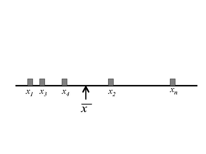
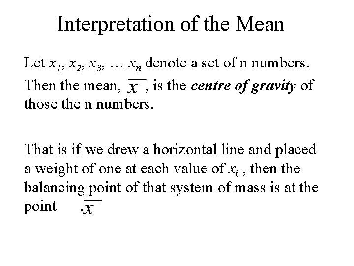
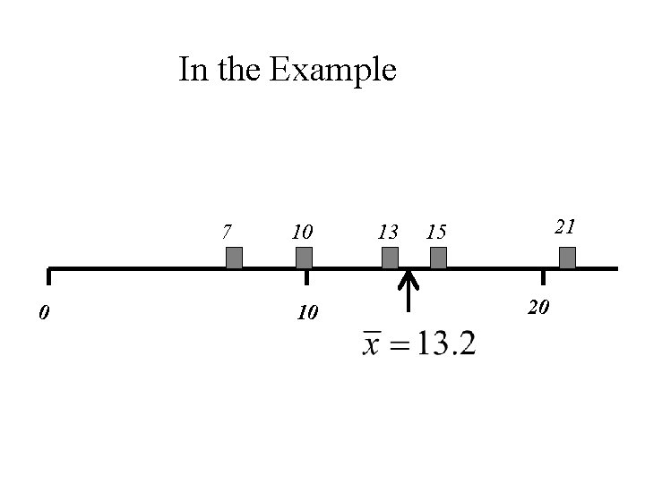
Interpretation of the Mean Let x 1, x 2, x 3, … xn denote a set of n numbers. Then the mean, , is the centre of gravity of those the n numbers. That is if we drew a horizontal line and placed a weight of one at each value of xi , then the balancing point of that system of mass is at the point.

x 1 x 3 x 4 x 2 xn

In the Example 7 0 10 10 13 21 15 20

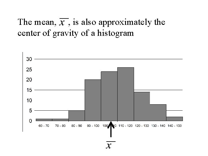
The mean, , is also approximately the center of gravity of a histogram

Measures of Central Location (Median)

The Median Let x 1, x 2, x 3, … xn denote a set of n numbers. Then the median of the n numbers is defined as the number that splits the numbers into two equal parts. To evaluate the median we arrange the numbers in increasing order.

If the number of observations is odd there will be one observation in the middle. This number is the median. If the number of observations is even there will be two middle observations. The median is the average of these two observations

Example Again let x 1, x 2, x 3 , x 4, x 5 denote a set of 5 denote the set of numbers in the following table. i 1 2 3 4 5 xi 10 15 21 7 13

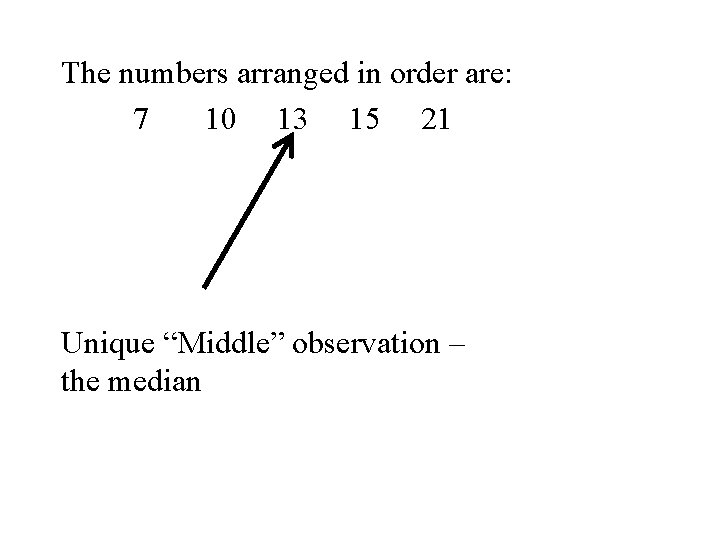
The numbers arranged in order are: 7 10 13 15 21 Unique “Middle” observation – the median

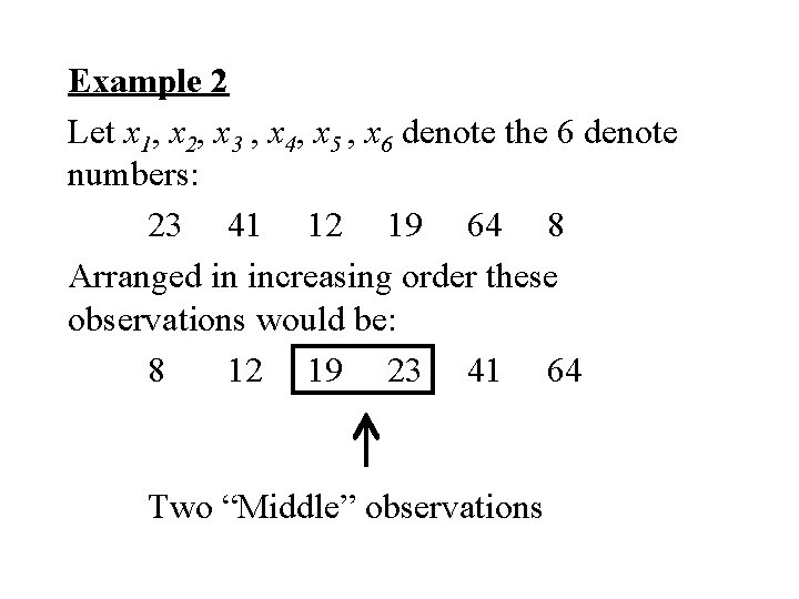
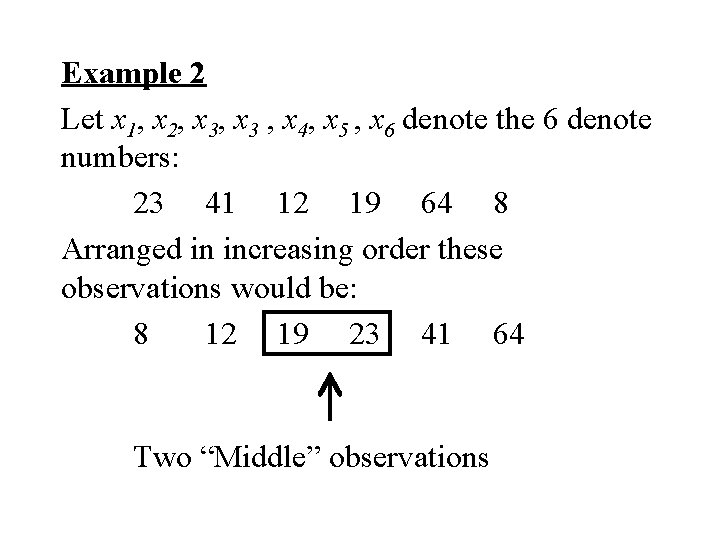
Example 2 Let x 1, x 2, x 3 , x 4, x 5 , x 6 denote the 6 denote numbers: 23 41 12 19 64 8 Arranged in increasing order these observations would be: 8 12 19 23 41 64 Two “Middle” observations

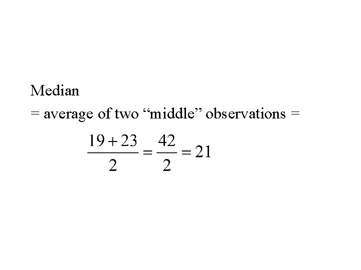
Median = average of two “middle” observations =

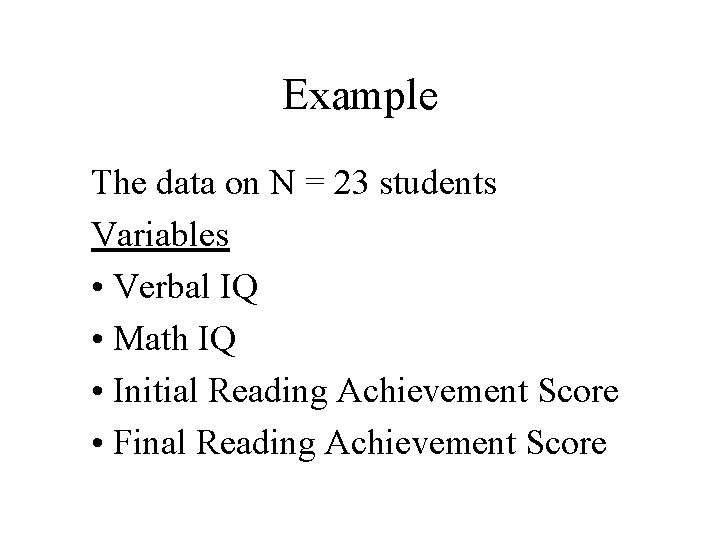
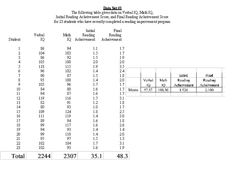
Example The data on N = 23 students Variables • Verbal IQ • Math IQ • Initial Reading Achievement Score • Final Reading Achievement Score

Data Set #3 The following table gives data on Verbal IQ, Math IQ, Initial Reading Acheivement Score, and Final Reading Acheivement Score for 23 students who have recently completed a reading improvement program Student Verbal IQ Math IQ 1 2 3 4 5 6 7 8 9 10 11 12 13 14 15 16 17 18 19 20 21 22 23 86 104 86 105 118 96 90 95 105 84 94 119 82 80 109 111 89 99 94 99 95 102 94 103 92 100 115 102 87 100 96 80 87 116 91 93 124 119 94 117 93 110 97 104 93 Initial Reading Acheivement 1. 1 1. 5 2. 0 1. 9 1. 4 1. 5 1. 4 1. 7 1. 6 1. 7 1. 2 1. 0 1. 8 1. 4 1. 6 1. 4 1. 5 1. 7 1. 6 Final Reading Acheivement 1. 7 1. 9 2. 0 3. 5 2. 4 1. 8 2. 0 1. 7 3. 1 1. 8 1. 7 2. 5 3. 0 1. 8 2. 6 1. 4 2. 0 1. 3 3. 1 1. 9

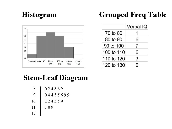
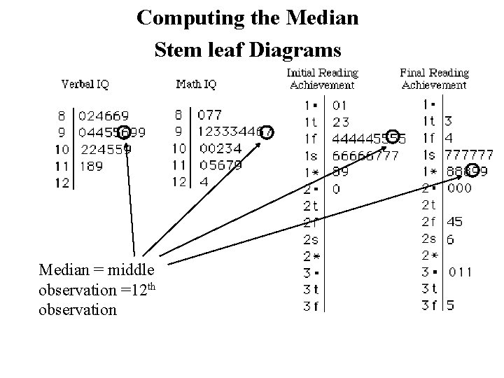
Computing the Median Stem leaf Diagrams Median = middle observation =12 th observation

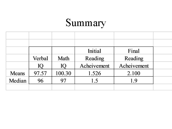
Summary

Numerical Measures

Numerical Measures • • Measures of Central Tendency (Location) Measures of Non Central Location Measure of Variability (Dispersion, Spread) Measures of Shape

Measures of Central Tendency (Location) • Mean • Median • Mode Central Location

Measures of Non-central Location • Quartiles, Mid-Hinges • Percentiles Non - Central Location

Measure of Variability (Dispersion, Spread) • Variance, standard deviation • Range • Inter-Quartile Range Variability

Measures of Shape • Skewness • Kurtosis

Measures of Central Location Mean Median

Mean Let x 1, x 2, x 3, … xn denote a set of n numbers. Then the mean of the n numbers is defined as:

The Median Let x 1, x 2, x 3, … xn denote a set of n numbers. Then the median of the n numbers is defined as the number that splits the numbers into two equal parts. To evaluate the median we arrange the numbers in increasing order.

If the number of observations is odd there will be one observation in the middle. This number is the median. If the number of observations is even there will be two middle observations. The median is the average of these two observations

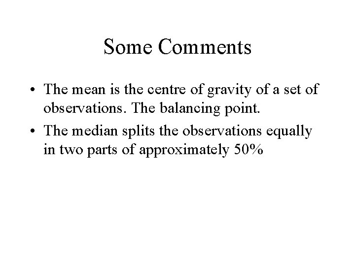
Some Comments • The mean is the centre of gravity of a set of observations. The balancing point. • The median splits the obsevations equally in two parts of approximately 50%

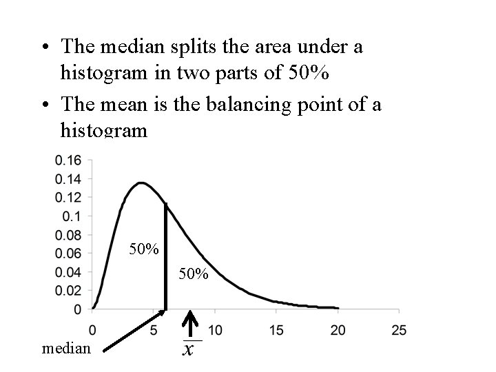
• The median splits the area under a histogram in two parts of 50% • The mean is the balancing point of a histogram 50% median

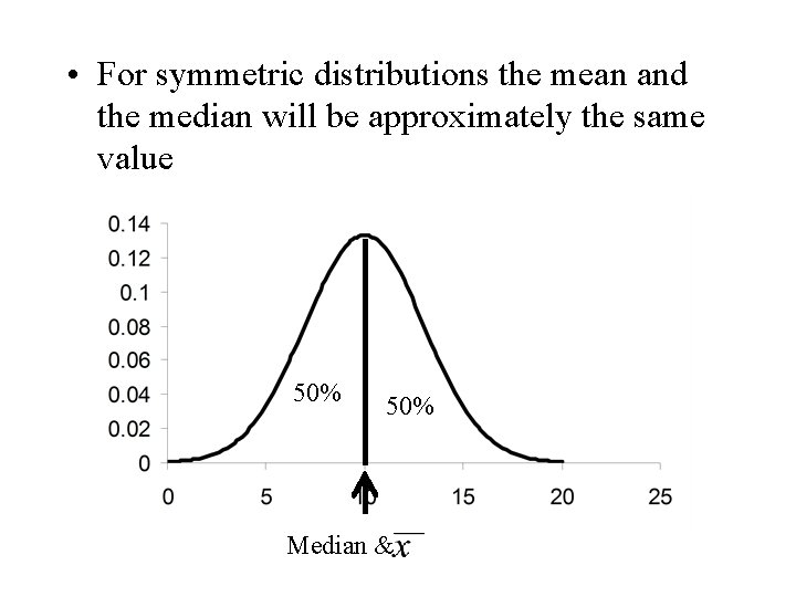
• For symmetric distributions the mean and the median will be approximately the same value 50% Median &

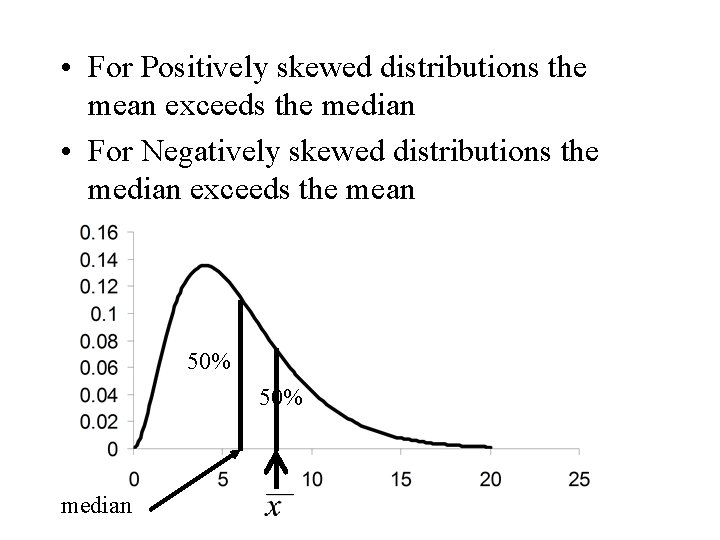
• For Positively skewed distributions the mean exceeds the median • For Negatively skewed distributions the median exceeds the mean 50% median

• An outlier is a “wild” observation in the data • Outliers occur because – of errors (typographical and computational) – Extreme cases in the population

• The mean is altered to a significant degree by the presence of outliers • Outliers have little effect on the value of the median • This is a reason for using the median in place of the mean as a measure of central location • Alternatively the mean is the best measure of central location when the data is Normally distributed (Bell-shaped)

Review

Summarizing Data Graphical Methods

Histogram Stem-Leaf Diagram Grouped Freq Table

Numerical Measures • • Measures of Central Tendency (Location) Measures of Non Central Location Measure of Variability (Dispersion, Spread) Measures of Shape The objective is to reduce the data to a small number of values that completely describe the data and certain aspects of the data.

Summation Notation Final value for i each term of the sum Quantity changing in each term of the sum Starting value for i

Example Let x 1, x 2, x 3, x 4, x 5 denote a set of 5 denote the set of numbers in the following table. i 1 2 3 4 5 xi 10 15 21 7 13

Then the symbol denotes the sum of these 3 numbers = 153 + 213 + 73 = 3375 + 9261 + 343 = 12979

Then the symbol denotes the sum of these 5 numbers x 1 + x 2 + x 3 + x 4 + x 5 = 10 + 15 + 21 + 7 + 13 = 66

Measures of Central Location (Mean)

Mean Let x 1, x 2, x 3, … xn denote a set of n numbers. Then the mean of the n numbers is defined as:

Example Again let x 1, x 2, x 3 , x 4, x 5 denote a set of 5 denote the set of numbers in the following table. i 1 2 3 4 5 xi 10 15 21 7 13

Then the mean of the 5 numbers is:

Interpretation of the Mean Let x 1, x 2, x 3, … xn denote a set of n numbers. Then the mean, , is the centre of gravity of those the n numbers. That is if we drew a horizontal line and placed a weight of one at each value of xi , then the balancing point of that system of mass is at the point.

x 1 x 3 x 4 x 2 xn

In the Example 7 0 10 10 13 21 15 20

The mean, , is also approximately the center of gravity of a histogram

The Median Let x 1, x 2, x 3, … xn denote a set of n numbers. Then the median of the n numbers is defined as the number that splits the numbers into two equal parts. To evaluate the median we arrange the numbers in increasing order.

If the number of observations is odd there will be one observation in the middle. This number is the median. If the number of observations is even there will be two middle observations. The median is the average of these two observations

Example Again let x 1, x 2, x 3 , x 4, x 5 denote a set of 5 denote the set of numbers in the following table. i 1 2 3 4 5 xi 10 15 21 7 13

The numbers arranged in order are: 7 10 13 15 21 Unique “Middle” observation – the median

Example 2 Let x 1, x 2, x 3 , x 4, x 5 , x 6 denote the 6 denote numbers: 23 41 12 19 64 8 Arranged in increasing order these observations would be: 8 12 19 23 41 64 Two “Middle” observations

Median = average of two “middle” observations =

Example The data on N = 23 students Variables • Verbal IQ • Math IQ • Initial Reading Achievement Score • Final Reading Achievement Score

Data Set #3 The following table gives data on Verbal IQ, Math IQ, Initial Reading Acheivement Score, and Final Reading Acheivement Score for 23 students who have recently completed a reading improvement program Student Verbal IQ Math IQ 1 2 3 4 5 6 7 8 9 10 11 12 13 14 15 16 17 18 19 20 21 22 23 86 104 86 105 118 96 90 95 105 84 94 119 82 80 109 111 89 99 94 99 95 102 94 103 92 100 115 102 87 100 96 80 87 116 91 93 124 119 94 117 93 110 97 104 93 Initial Reading Acheivement 1. 1 1. 5 2. 0 1. 9 1. 4 1. 5 1. 4 1. 7 1. 6 1. 7 1. 2 1. 0 1. 8 1. 4 1. 6 1. 4 1. 5 1. 7 1. 6 Final Reading Acheivement 1. 7 1. 9 2. 0 3. 5 2. 4 1. 8 2. 0 1. 7 3. 1 1. 8 1. 7 2. 5 3. 0 1. 8 2. 6 1. 4 2. 0 1. 3 3. 1 1. 9

Computing the Median Stem leaf Diagrams Median = middle observation =12 th observation

Summary

Some Comments • The mean is the centre of gravity of a set of observations. The balancing point. • The median splits the observations equally in two parts of approximately 50%

• The median splits the area under a histogram in two parts of 50% • The mean is the balancing point of a histogram 50% median

• For symmetric distributions the mean and the median will be approximately the same value 50% Median &

• For Positively skewed distributions the mean exceeds the median • For Negatively skewed distributions the median exceeds the mean 50% median

• An outlier is a “wild” observation in the data • Outliers occur because – of errors (typographical and computational) – Extreme cases in the population

• The mean is altered to a significant degree by the presence of outliers • Outliers have little effect on the value of the median • This is a reason for using the median in place of the mean as a measure of central location • Alternatively the mean is the best measure of central location when the data is Normally distributed (Bell-shaped)

Measures of Non-Central Location • • Percentiles Quartiles (Hinges, Mid-hinges)

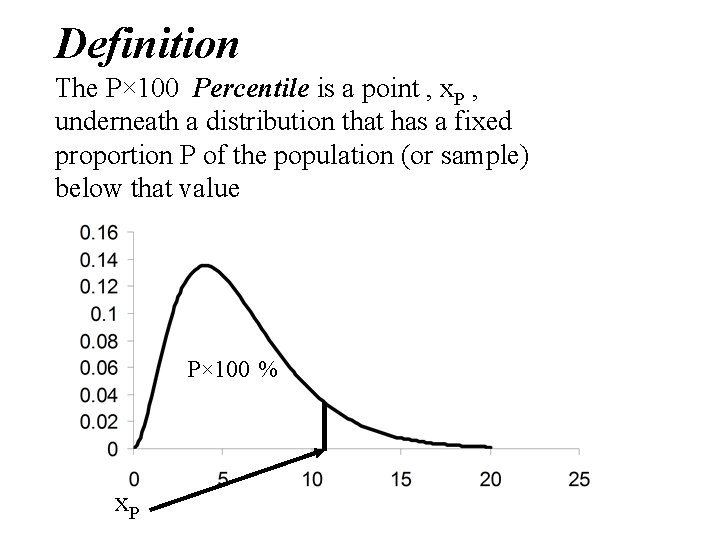
Definition The P× 100 Percentile is a point , x. P , underneath a distribution that has a fixed proportion P of the population (or sample) below that value P× 100 % x. P

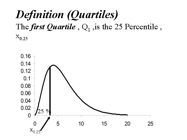
Definition (Quartiles) The first Quartile , Q 1 , is the 25 Percentile , x 0. 25 25 % x 0. 25

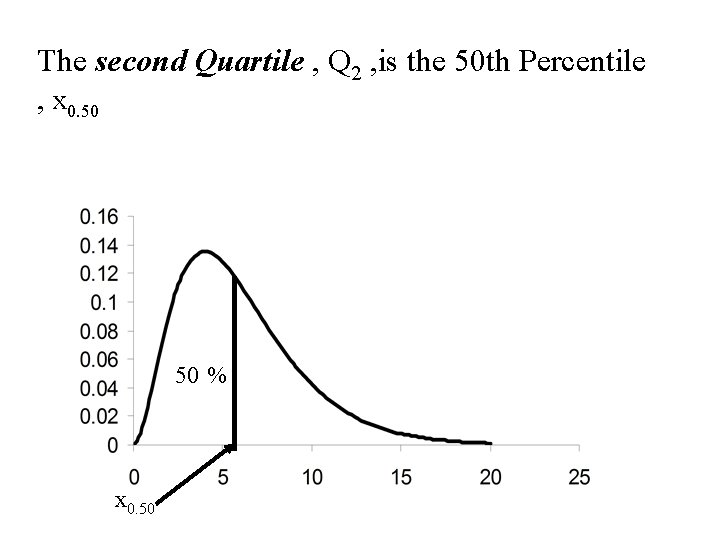
The second Quartile , Q 2 , is the 50 th Percentile , x 0. 50 50 % x 0. 50

• The second Quartile , Q 2 , is also the median and the 50 th percentile

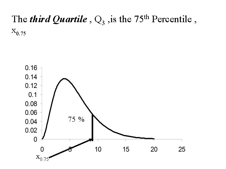
The third Quartile , Q 3 , is the 75 th Percentile , x 0. 75 75 % x 0. 75

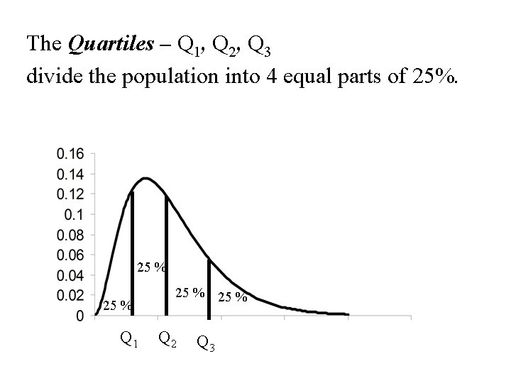
The Quartiles – Q 1, Q 2, Q 3 divide the population into 4 equal parts of 25%. 25 % Q 1 25 % Q 2 Q 3

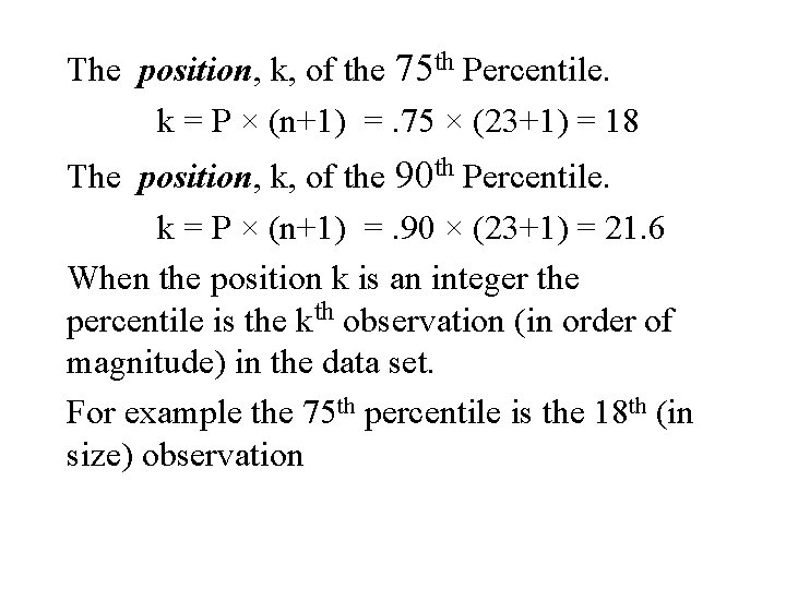
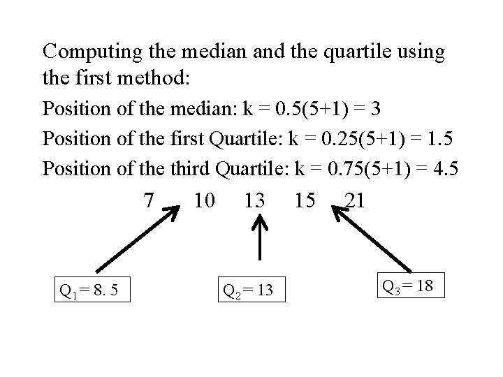
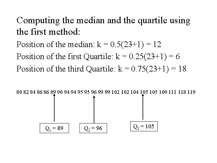
Computing Percentiles and Quartiles – Method 1 • The first step is to order the observations in increasing order. • We then compute the position, k, of the P× 100 Percentile. k = P × (n+1) Where n = the number of observations

Example The data on n = 23 students Variables • Verbal IQ • Math IQ • Initial Reading Achievement Score • Final Reading Achievement Score We want to compute the 75 th percentile and the 90 th percentile

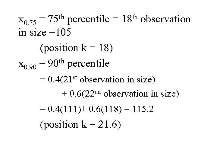
The position, k, of the 75 th Percentile. k = P × (n+1) =. 75 × (23+1) = 18 The position, k, of the 90 th Percentile. k = P × (n+1) =. 90 × (23+1) = 21. 6 When the position k is an integer the percentile is the kth observation (in order of magnitude) in the data set. For example the 75 th percentile is the 18 th (in size) observation

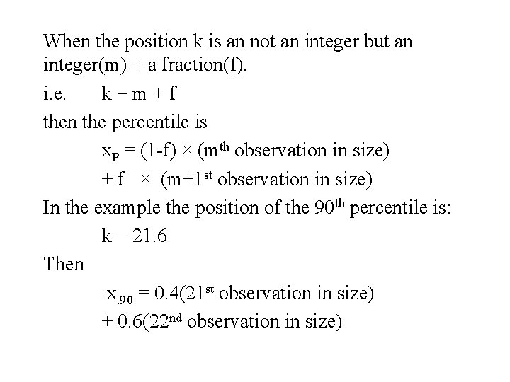
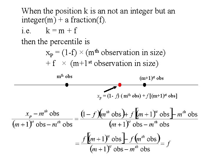
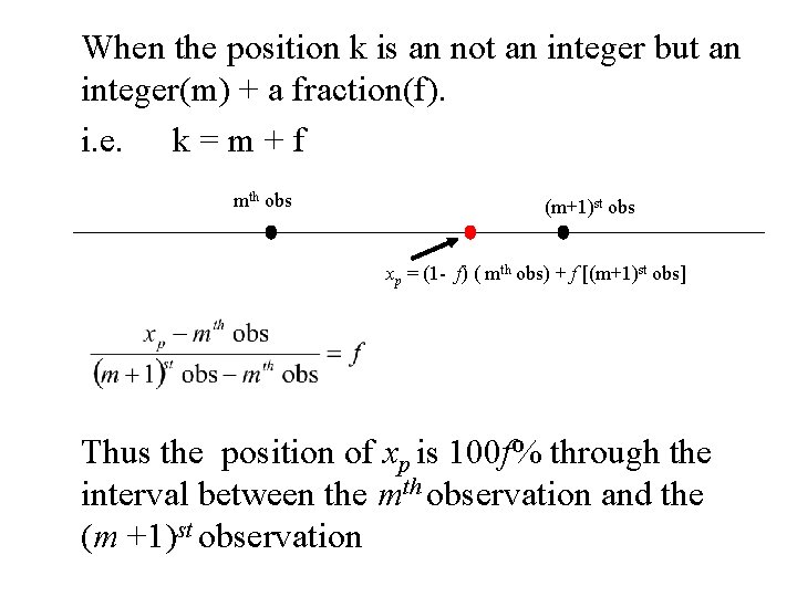
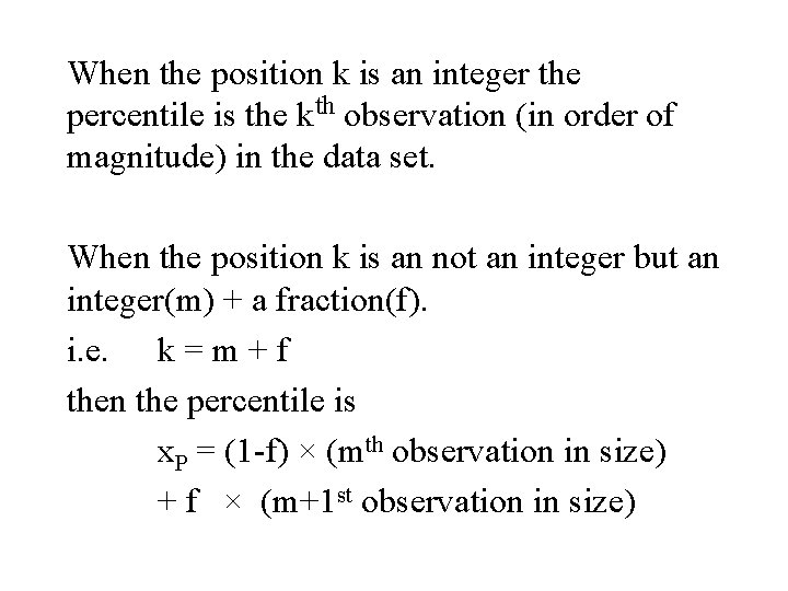
When the position k is an not an integer but an integer(m) + a fraction(f). i. e. k=m+f then the percentile is x. P = (1 -f) × (mth observation in size) + f × (m+1 st observation in size) In the example the position of the 90 th percentile is: k = 21. 6 Then x. 90 = 0. 4(21 st observation in size) + 0. 6(22 nd observation in size)

When the position k is an not an integer but an integer(m) + a fraction(f). i. e. k=m+f then the percentile is x. P = (1 -f) × (mth observation in size) + f × (m+1 st observation in size) mth obs (m+1)st obs xp = (1 - f) ( mth obs) + f [(m+1)st obs]

When the position k is an not an integer but an integer(m) + a fraction(f). i. e. k = m + f mth obs (m+1)st obs xp = (1 - f) ( mth obs) + f [(m+1)st obs] Thus the position of xp is 100 f% through the interval between the mth observation and the (m +1)st observation

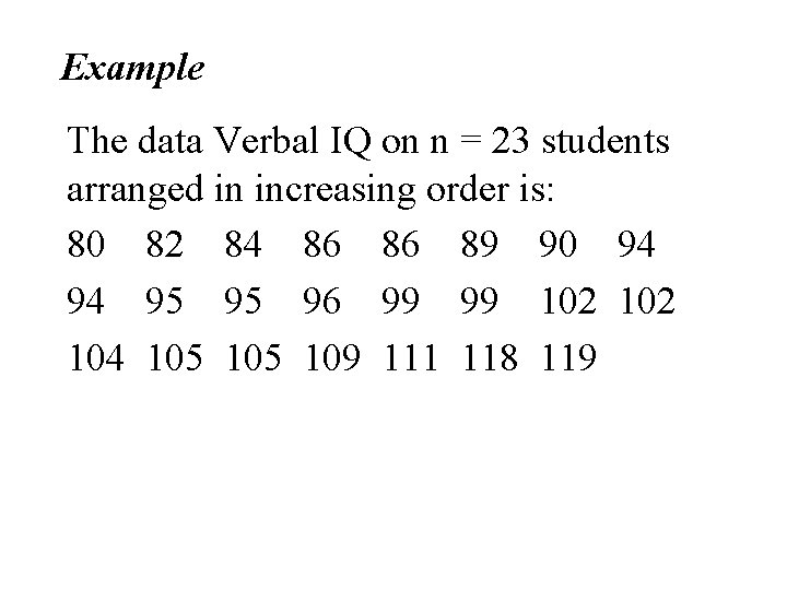
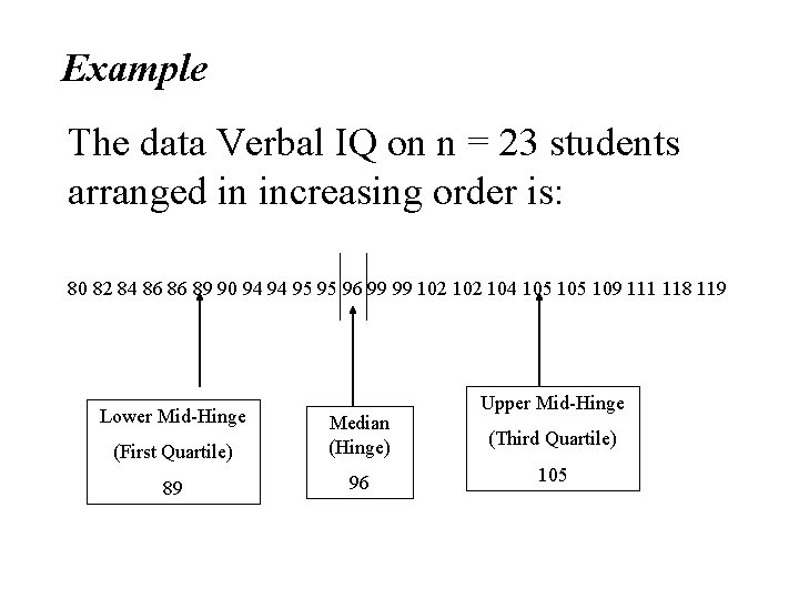
Example The data Verbal IQ on n = 23 students arranged in increasing order is: 80 82 84 86 86 89 90 94 94 95 95 96 99 99 102 104 105 109 111 118 119

x 0. 75 = 75 th percentile = 18 th observation in size =105 (position k = 18) x 0. 90 = 90 th percentile = 0. 4(21 st observation in size) + 0. 6(22 nd observation in size) = 0. 4(111)+ 0. 6(118) = 115. 2 (position k = 21. 6)

An Alternative method for computing Quartiles – Method 2 • Sometimes this method will result in the same values for the quartiles. • Sometimes this method will result in the different values for the quartiles. • For large samples the two methods will result in approximately the same answer.

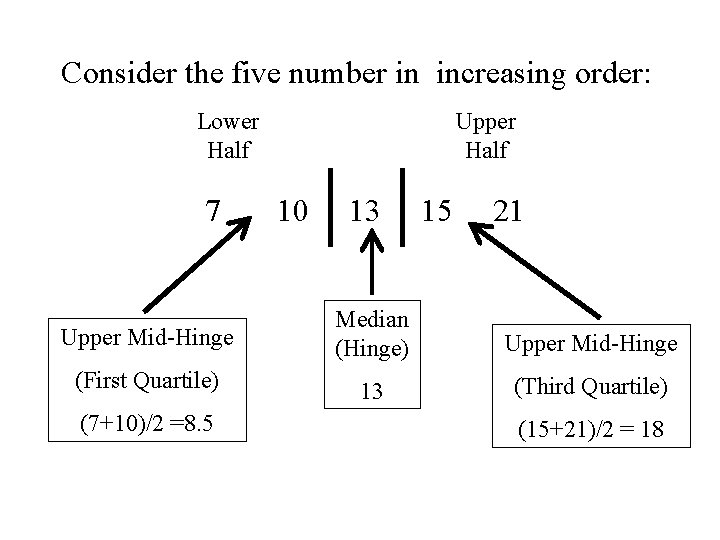
Let x 1, x 2, x 3, … xn denote a set of n numbers. The first step in Method 2 is to arrange the numbers in increasing order. From the arranged numbers we compute the median. This is also called the Hinge

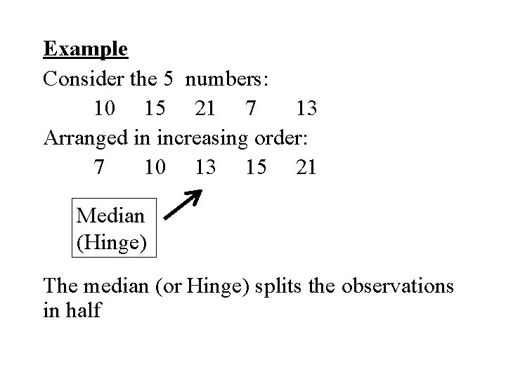
Example Consider the 5 numbers: 10 15 21 7 13 Arranged in increasing order: 7 10 13 15 21 Median (Hinge) The median (or Hinge) splits the observations in half

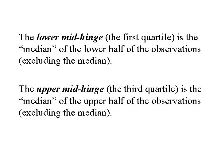
The lower mid-hinge (the first quartile) is the “median” of the lower half of the observations (excluding the median). The upper mid-hinge (the third quartile) is the “median” of the upper half of the observations (excluding the median).

Consider the five number in increasing order: Lower Half 7 Upper Half 10 13 15 21 Upper Mid-Hinge Median (Hinge) Upper Mid-Hinge (First Quartile) 13 (Third Quartile) (7+10)/2 =8. 5 (15+21)/2 = 18

Computing the median and the quartile using the first method: Position of the median: k = 0. 5(5+1) = 3 Position of the first Quartile: k = 0. 25(5+1) = 1. 5 Position of the third Quartile: k = 0. 75(5+1) = 4. 5 7 Q 1 = 8. 5 10 13 Q 2 = 13 15 21 Q 3 = 18

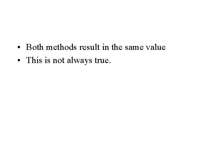
• Both methods result in the same value • This is not always true.

Example The data Verbal IQ on n = 23 students arranged in increasing order is: 80 82 84 86 86 89 90 94 94 95 95 96 99 99 102 104 105 109 111 118 119 Lower Mid-Hinge (First Quartile) Median (Hinge) 89 96 Upper Mid-Hinge (Third Quartile) 105

Computing the median and the quartile using the first method: Position of the median: k = 0. 5(23+1) = 12 Position of the first Quartile: k = 0. 25(23+1) = 6 Position of the third Quartile: k = 0. 75(23+1) = 18 80 82 84 86 86 89 90 94 94 95 95 96 99 99 102 104 105 109 111 118 119 Q 1 = 89 Q 2 = 96 Q 3 = 105

• Many programs compute percentiles, quartiles etc. • Each may use different methods. • It is important to know which method is being used. • The different methods result in answers that are close when the sample size is large.

Measures of Central Location Mean Median

Mean Let x 1, x 2, x 3, … xn denote a set of n numbers. Then the mean of the n numbers is defined as:

The Median Let x 1, x 2, x 3, … xn denote a set of n numbers. Then the median of the n numbers is defined as the number that splits the numbers into two equal parts. To evaluate the median we arrange the numbers in increasing order.

If the number of observations is odd there will be one observation in the middle. This number is the median. If the number of observations is even there will be two middle observations. The median is the average of these two observations

Measures of Non-Central Location • • Percentiles Quartiles (Hinges, Mid-hinges)

Definition The P× 100 Percentile is a point , x. P , underneath a distribution that has a fixed proportion P of the population (or sample) below that value P× 100 % x. P

Computing Percentiles and Quartiles – Method 1 • The first step is to order the observations in increasing order. • We then compute the position, k, of the P× 100 Percentile. k = P × (n+1) Where n = the number of observations

When the position k is an integer the percentile is the kth observation (in order of magnitude) in the data set. When the position k is an not an integer but an integer(m) + a fraction(f). i. e. k = m + f then the percentile is x. P = (1 -f) × (mth observation in size) + f × (m+1 st observation in size)

An Alternative method for computing Quartiles – Method 2 • Sometimes this method will result in the same values for the quartiles. • Sometimes this method will result in the different values for the quartiles. • For large samples the two methods will result in approximately the same answer.

Let x 1, x 2, x 3, … xn denote a set of n numbers. The first step in Method 2 is to arrange the numbers in increasing order. From the arranged numbers we compute the median. This is also called the Hinge

The lower mid-hinge (the first quartile) is the “median” of the lower half of the observations (excluding the median). The upper mid-hinge (the third quartile) is the “median” of the upper half of the observations (excluding the median).

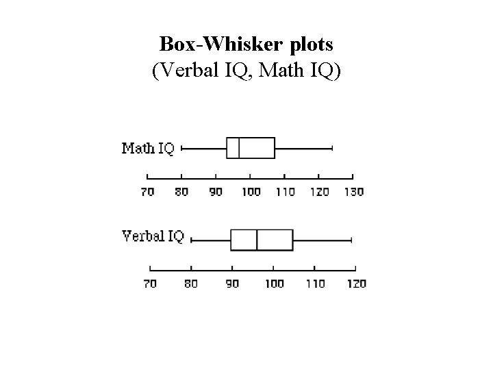
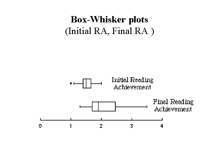
Box-Plots Box-Whisker Plots • A graphical method of of displaying data • An alternative to the histogram and stem-leaf diagram

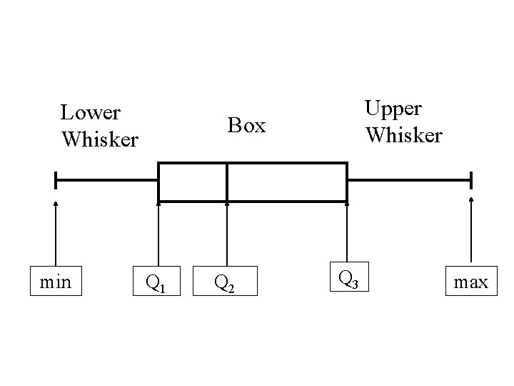
To Draw a Box Plot • Compute the Hinge (Median, Q 2) and the Mid-hinges (first & third quartiles – Q 1 and Q 3 ) • We also compute the largest and smallest of the observations – the max and the min.

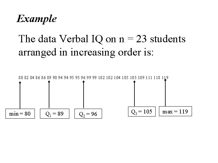
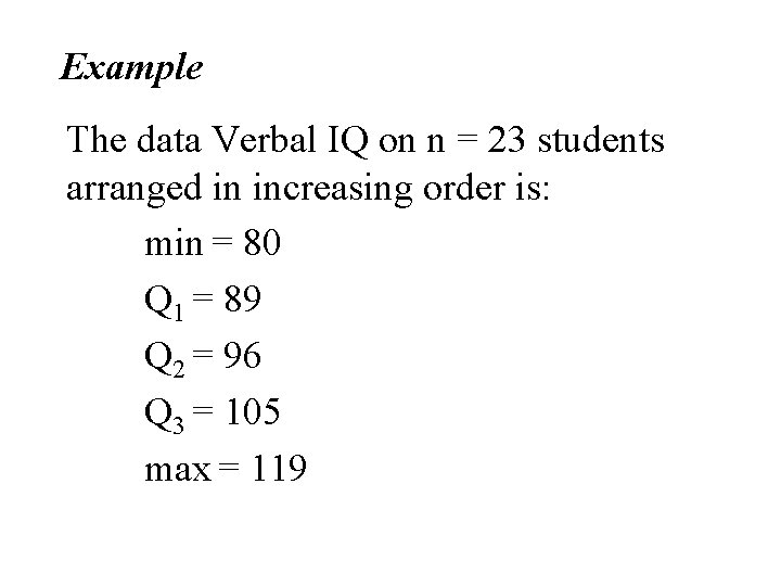
Example The data Verbal IQ on n = 23 students arranged in increasing order is: 80 82 84 86 86 89 90 94 94 95 95 96 99 99 102 104 105 109 111 118 119 min = 80 Q 1 = 89 Q 2 = 96 Q 3 = 105 max = 119

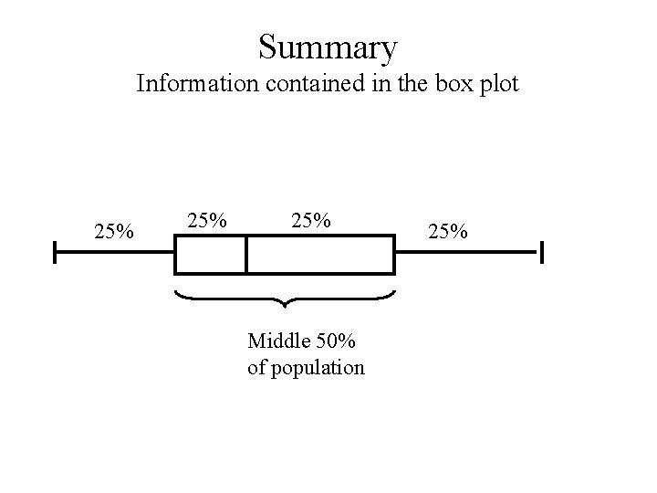
The Box Plot is then drawn • Drawing above an axis a “box” from Q 1 to Q 3. • Drawing vertical line in the box at the median, Q 2 • Drawing whiskers at the lower and upper ends of the box going down to the min and up to max.

Lower Whisker min Upper Whisker Box Q 1 Q 2 Q 3 max

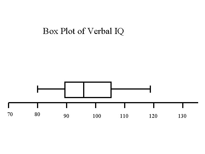
Example The data Verbal IQ on n = 23 students arranged in increasing order is: min = 80 Q 1 = 89 Q 2 = 96 Q 3 = 105 max = 119

Box Plot of Verbal IQ 70 80 90 100 110 120 130

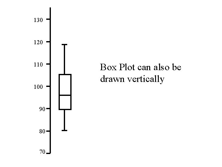
130 120 110 100 90 80 70 Box Plot can also be drawn vertically

Box-Whisker plots (Verbal IQ, Math IQ)

Box-Whisker plots (Initial RA, Final RA )

Summary Information contained in the box plot 25% 25% Middle 50% of population 25%

Next topic: Numerical Measures of Variability