Descriptive Statistics Central Tendency Central Tendency In general

Descriptive Statistics (Central Tendency)

Central Tendency • In general terms, central tendency is a statistical measure that determines a single value that accurately describes the center of the distribution and represents the entire distribution of scores. • The goal of central tendency is to identify the single value that is the best representative for the entire set of data. 2

Central Tendency (cont. ) • By identifying the "average score, " central tendency allows researchers to summarize or condense a large set of data into a single value. • Thus, central tendency serves as a descriptive statistic because it allows researchers to describe or present a set of data in a very simplified, concise form. • In addition, it is possible to compare two (or more) sets of data by simply comparing the average score (central tendency) for one set versus the average score for another set. 3

The Mean, the Median, and the Mode • It is essential that central tendency be determined by an objective and well‑defined procedure so that others will understand exactly how the "average" value was obtained and can duplicate the process. • No single procedure always produces a good, representative value. Therefore, researchers have developed three commonly used techniques for measuring central tendency: the mean, the median, and the mode. 4

The Mean • The mean is the most commonly used measure of central tendency. • Computation of the mean requires scores that are numerical values measured on an interval or ratio scale. • The mean is obtained by computing the sum, or total, for the entire set of scores, then dividing this sum by the number of scores. 5

The Mean (cont. ) Conceptually, the mean can also be defined as: 1. The mean is the amount that each individual receives when the total (ΣX) is divided equally among all individuals. 2. The mean is the balance point of the distribution because the sum of the distances below the mean is exactly equal to the sum of the distances above the mean. 6

Changing the Mean • Because the calculation of the mean involves every score in the distribution, changing the value of any score will change the value of the mean. • Modifying a distribution by discarding scores or by adding new scores will usually change the value of the mean. • To determine how the mean will be affected for any specific situation you must consider: 1) how the number of scores is affected, and 2) how the sum of the scores is affected. 7

Changing the Mean (cont. ) • If a constant value is added to every score in a distribution, then the same constant value is added to the mean. Also, if every score is multiplied by a constant value, then the mean is also multiplied by the same constant value. 8

When the Mean Won’t Work • Although the mean is the most commonly used measure of central tendency, there are situations where the mean does not provide a good, representative value, and there are situations where you cannot compute a mean at all. • When a distribution contains a few extreme scores (or is very skewed), the mean will be pulled toward the extremes (displaced toward the tail). In this case, the mean will not provide a "central" value correctly. 9

When the Mean Won’t Work (cont. ) • With data from a nominal scale it is impossible to compute a mean, and when data are measured on an ordinal scale (ranks), it is usually inappropriate to compute a mean. • Thus, the mean does not always work as a measure of central tendency and it is necessary to have alternative procedures available. 10

The Median • If the scores in a distribution are listed in order from smallest to largest, the median is defined as the midpoint of the list. • The median divides the scores so that 50% of the scores in the distribution have values that are equal to or less than the median. • Computation of the median requires scores that can be placed in rank order (smallest to largest) and are measured on an ordinal, interval, or ratio scale. 11

The Median (cont. ) Usually, the median can be found by a simple counting procedure: 1. With an odd number of scores, list the values in order, and the median is the middle score in the list. 2. With an even number of scores, list the values in order, and the median is half-way between the middle two scores. 12

The Median (cont. ) • If the scores are measurements of a continuous variable, it is possible to find the median by first placing the scores in a frequency distribution. • Determine the median rage • Use the formula for computing the value from median range 13

The Median (cont. ) • One advantage of the median is that it is relatively unaffected by extreme scores. • Thus, the median tends to stay in the "center" of the distribution even when there a few extreme scores or when the distribution is very skewed. In these situations, the median serves as a good alternative to the mean. 14

The Mode • The mode is defined as the most frequently occurring category or score in the distribution. • In a frequency distribution graph, the mode is the category or score corresponding to the peak or high point of the distribution. • The mode can be determined for data measured on any scale of measurement: nominal, ordinal, interval, or ratio. 15

The Mode (cont. ) • The primary value of the mode is that it is the only measure of central tendency that can be used for data measured on a nominal scale. In addition, the mode often is used as a supplemental measure of central tendency that is reported along with the mean or the median. 16

Bimodal Distributions • It is possible for a distribution to have more than one mode. Such a distribution is called bimodal. (Note that a distribution can have only one mean and only one median. ) • In addition, the term "mode" is often used to describe a peak in a distribution that is not really the highest point. Thus, a distribution may have a major mode at the highest peak and a minor mode at a secondary peak in a different location. 17

Central Tendency and the Shape of the Distribution • Because the mean, the median, and the mode are all measuring central tendency, the three measures are often systematically related to each other. • In a symmetrical distribution, for example, the mean and median will always be equal. 18

Central Tendency and the Shape of the Distribution (cont. ) • If a symmetrical distribution has only one mode, the mode, mean, and median will all have the same value. • In a skewed distribution, the mode will be located at the peak on one side and the mean usually will be displaced toward the tail on the other side. • The median is usually located between the mean and the mode. 19

Reporting Central Tendency in Research Reports • In manuscripts and in published research reports, the sample mean is identified with the letter. • There is no standardized notation for reporting the median or the mode. • In research situations where several means are obtained for different groups or for different treatment conditions, it is common to present all of the means in a single graph. 20

Reporting Central Tendency in Research Reports (cont. ) • The different groups or treatment conditions are listed along the horizontal axis and the means are displayed by a bar or a point above each of the groups. • The height of the bar (or point) indicates the value of the mean for each group. Similar graphs are also used to show several medians in one display. 21

Numerical Descriptive Measures

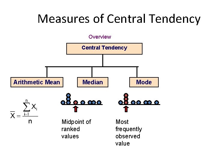
Measures of Central Tendency Overview Central Tendency Arithmetic Mean Median Midpoint of ranked values Mode Most frequently observed value

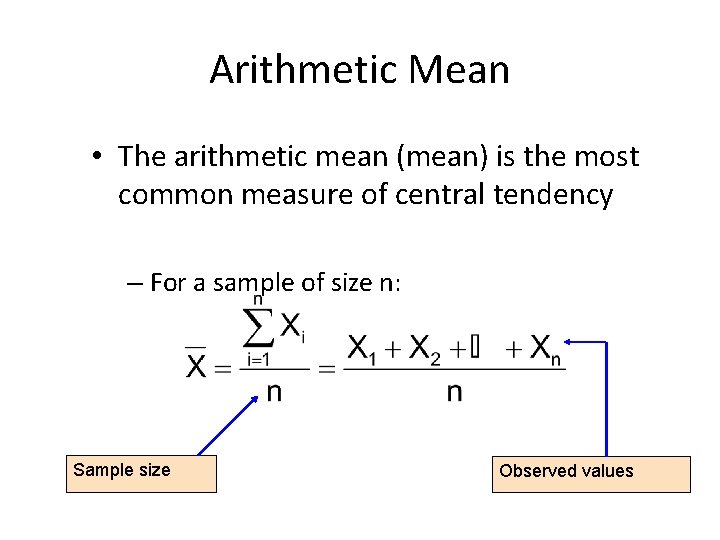
Arithmetic Mean • The arithmetic mean (mean) is the most common measure of central tendency – For a sample of size n: Sample size Observed values

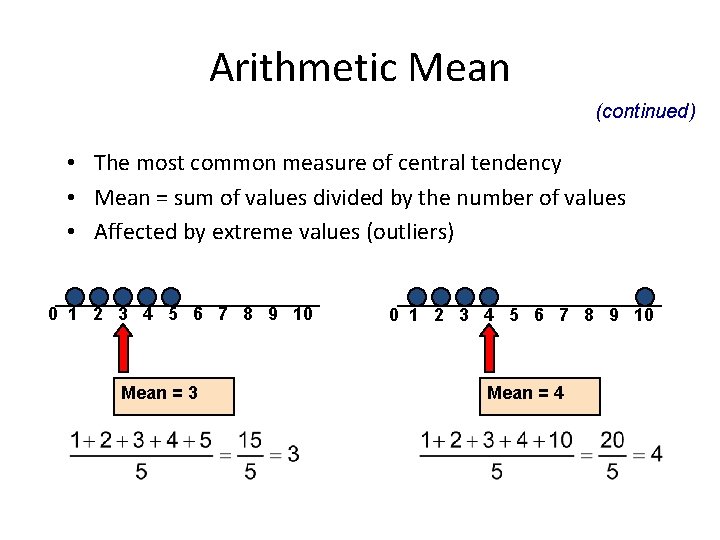
Arithmetic Mean (continued) • The most common measure of central tendency • Mean = sum of values divided by the number of values • Affected by extreme values (outliers) 0 1 2 3 4 5 6 7 8 9 10 Mean = 3 0 1 2 3 4 5 6 7 8 9 10 Mean = 4

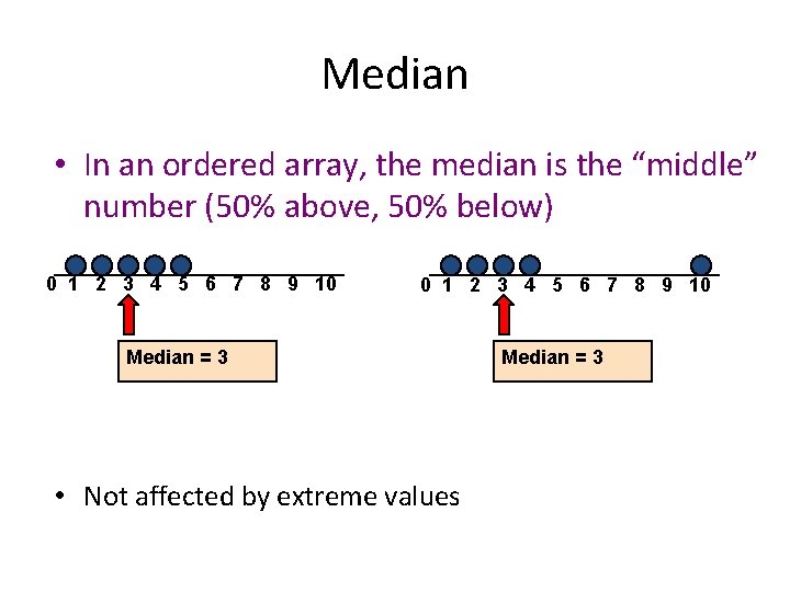
Median • In an ordered array, the median is the “middle” number (50% above, 50% below) 0 1 2 3 4 5 6 7 8 9 10 Median = 3 • Not affected by extreme values Median = 3

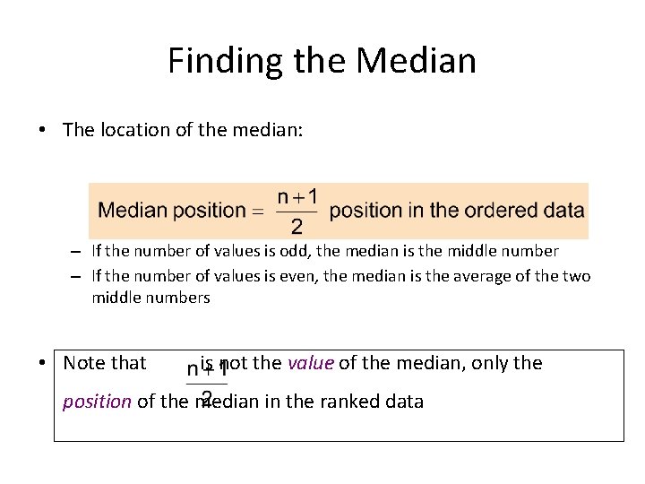
Finding the Median • The location of the median: – If the number of values is odd, the median is the middle number – If the number of values is even, the median is the average of the two middle numbers • Note that is not the value of the median, only the position of the median in the ranked data

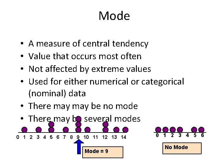
Mode A measure of central tendency Value that occurs most often Not affected by extreme values Used for either numerical or categorical (nominal) data • There may be no mode • There may be several modes • • 0 1 2 3 4 5 6 7 8 9 10 11 12 13 14 Mode = 9 0 1 2 3 4 5 6 No Mode

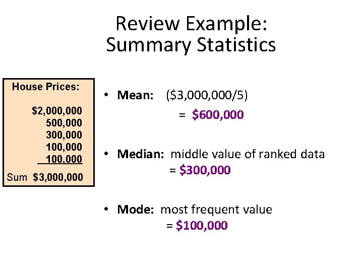
Review Example: Summary Statistics House Prices: $2, 000 500, 000 300, 000 100, 000 Sum $3, 000 • Mean: ($3, 000/5) = $600, 000 • Median: middle value of ranked data = $300, 000 • Mode: most frequent value = $100, 000

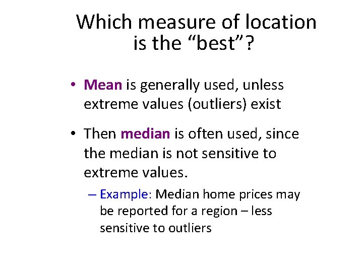
Which measure of location is the “best”? • Mean is generally used, unless extreme values (outliers) exist • Then median is often used, since the median is not sensitive to extreme values. – Example: Median home prices may be reported for a region – less sensitive to outliers

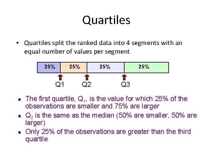
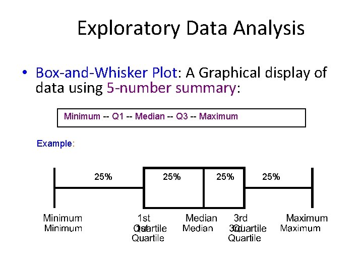
Quartiles • Quartiles split the ranked data into 4 segments with an equal number of values per segment 25% Q 1 n n n 25% Q 2 25% Q 3 The first quartile, Q 1, is the value for which 25% of the observations are smaller and 75% are larger Q 2 is the same as the median (50% are smaller, 50% are larger) Only 25% of the observations are greater than the third quartile

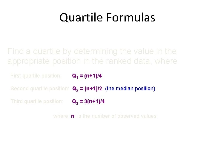
Quartile Formulas Find a quartile by determining the value in the appropriate position in the ranked data, where First quartile position: Q 1 = (n+1)/4 Second quartile position: Q 2 = (n+1)/2 (the median position) Third quartile position: Q 3 = 3(n+1)/4 where n is the number of observed values

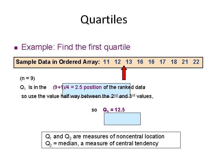
Quartiles n Example: Find the first quartile Sample Data in Ordered Array: 11 12 13 16 16 17 18 21 22 (n = 9) Q 1 is in the (9+1)/4 = 2. 5 position of the ranked data so use the value half way between the 2 nd and 3 rd values, so Q 1 = 12. 5 Q 1 and Q 3 are measures of noncentral location Q 2 = median, a measure of central tendency

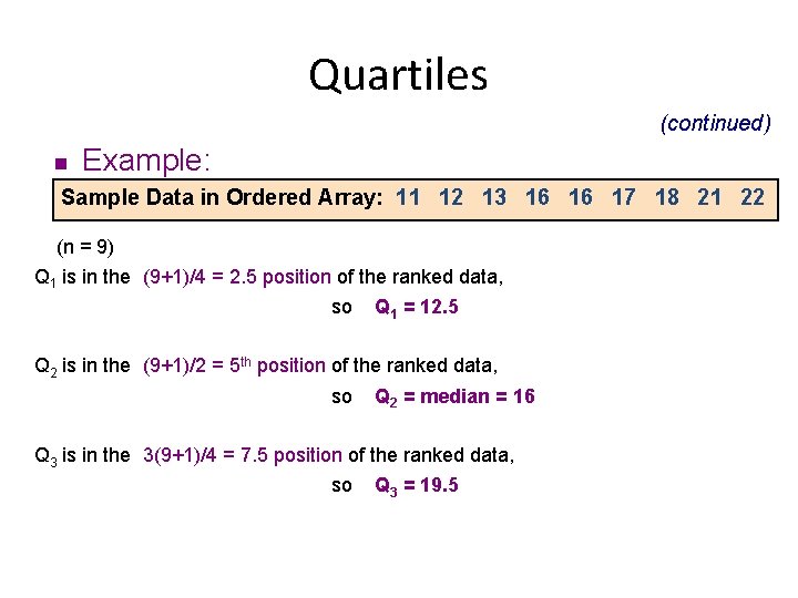
Quartiles (continued) n Example: Sample Data in Ordered Array: 11 12 13 16 16 17 18 21 22 (n = 9) Q 1 is in the (9+1)/4 = 2. 5 position of the ranked data, so Q 1 = 12. 5 Q 2 is in the (9+1)/2 = 5 th position of the ranked data, so Q 2 = median = 16 Q 3 is in the 3(9+1)/4 = 7. 5 position of the ranked data, so Q 3 = 19. 5

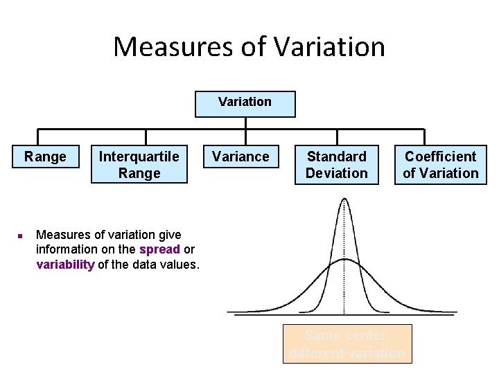
Measures of Variation Range n Interquartile Range Variance Standard Deviation Coefficient of Variation Measures of variation give information on the spread or variability of the data values. Same center, different variation

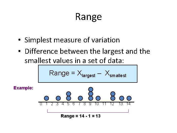
Range • Simplest measure of variation • Difference between the largest and the smallest values in a set of data: Range = Xlargest – Xsmallest Example: 0 1 2 3 4 5 6 7 8 9 10 11 12 Range = 14 - 1 = 13 13 14

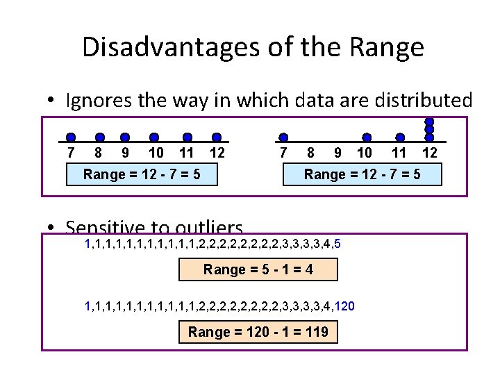
Disadvantages of the Range • Ignores the way in which data are distributed 7 8 9 10 11 12 Range = 12 - 7 = 5 7 8 9 10 11 Range = 12 - 7 = 5 • Sensitive to outliers 1, 1, 1, 2, 2, 3, 3, 4, 5 Range = 5 - 1 = 4 1, 1, 1, 2, 2, 3, 3, 4, 120 Range = 120 - 1 = 119 12

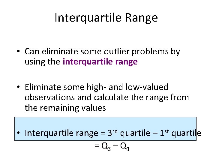
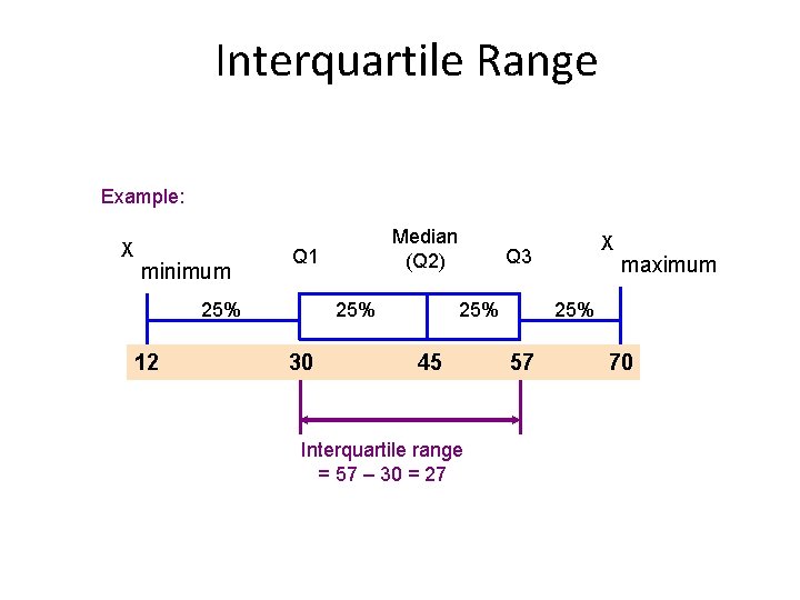
Interquartile Range • Can eliminate some outlier problems by using the interquartile range • Eliminate some high- and low-valued observations and calculate the range from the remaining values • Interquartile range = 3 rd quartile – 1 st quartile = Q 3 – Q 1

Interquartile Range Example: X minimum Q 1 25% 12 Median (Q 2) 25% 30 X Q 3 25% 45 Interquartile range = 57 – 30 = 27 maximum 25% 57 70

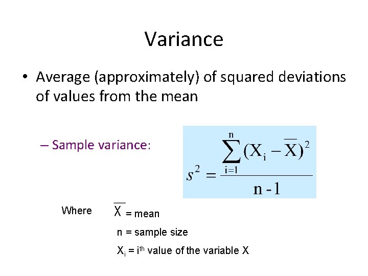
Variance • Average (approximately) of squared deviations of values from the mean – Sample variance: Where = mean n = sample size Xi = ith value of the variable X

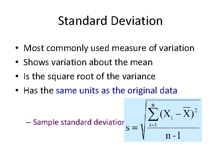
Standard Deviation • • Most commonly used measure of variation Shows variation about the mean Is the square root of the variance Has the same units as the original data – Sample standard deviation:

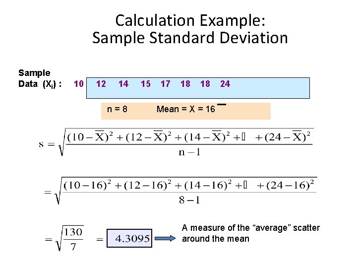
Calculation Example: Sample Standard Deviation Sample Data (Xi) : 10 12 14 n=8 15 17 18 18 24 Mean = X = 16 A measure of the “average” scatter around the mean

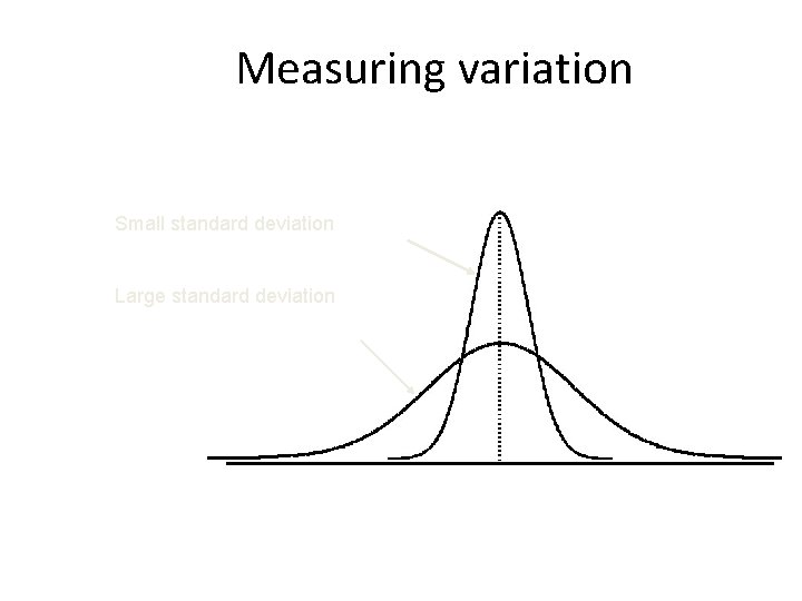
Measuring variation Small standard deviation Large standard deviation

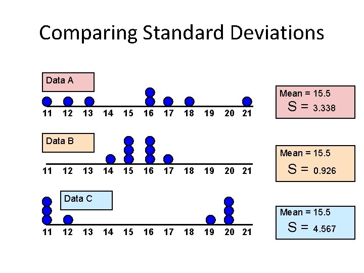
Comparing Standard Deviations Data A Mean = 15. 5 11 12 13 14 15 16 17 18 19 20 21 S = 3. 338 Data B Mean = 15. 5 11 12 13 14 15 16 17 18 19 20 21 S = 0. 926 Data C Mean = 15. 5 11 12 13 14 15 16 17 18 19 20 21 S = 4. 567

Advantages of Variance and Standard Deviation • Each value in the data set is used in the calculation • Values far from the mean are given extra weight (because deviations from the mean are squared)

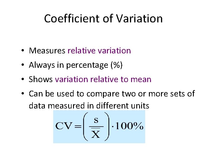
Coefficient of Variation • Measures relative variation • Always in percentage (%) • Shows variation relative to mean • Can be used to compare two or more sets of data measured in different units

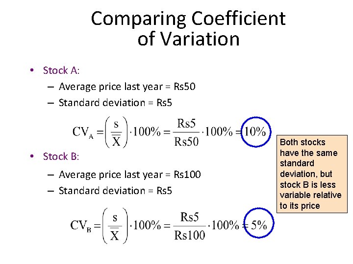
Comparing Coefficient of Variation • Stock A: – Average price last year = Rs 50 – Standard deviation = Rs 5 • Stock B: – Average price last year = Rs 100 – Standard deviation = Rs 5 Both stocks have the same standard deviation, but stock B is less variable relative to its price

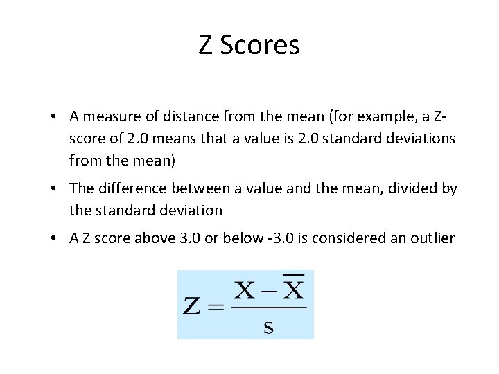
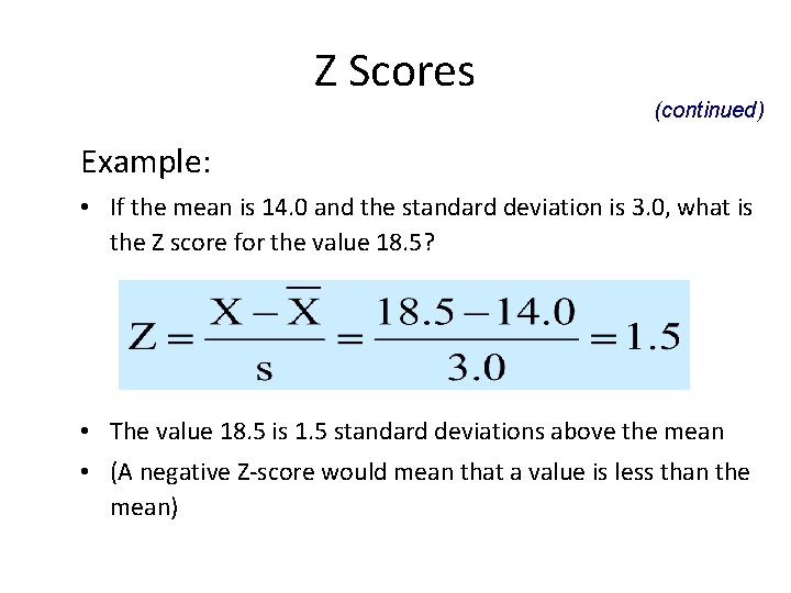
Z Scores • A measure of distance from the mean (for example, a Zscore of 2. 0 means that a value is 2. 0 standard deviations from the mean) • The difference between a value and the mean, divided by the standard deviation • A Z score above 3. 0 or below -3. 0 is considered an outlier

Z Scores (continued) Example: • If the mean is 14. 0 and the standard deviation is 3. 0, what is the Z score for the value 18. 5? • The value 18. 5 is 1. 5 standard deviations above the mean • (A negative Z-score would mean that a value is less than the mean)

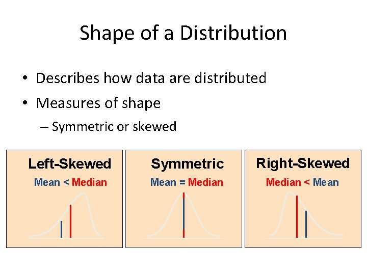
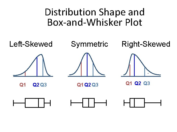
Shape of a Distribution • Describes how data are distributed • Measures of shape – Symmetric or skewed Left-Skewed Symmetric Right-Skewed Mean < Median Mean = Median < Mean

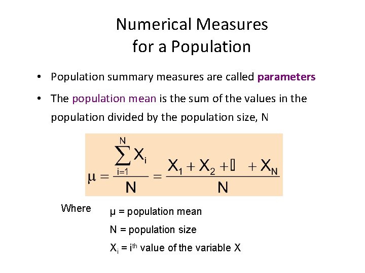
Numerical Measures for a Population • Population summary measures are called parameters • The population mean is the sum of the values in the population divided by the population size, N Where μ = population mean N = population size Xi = ith value of the variable X

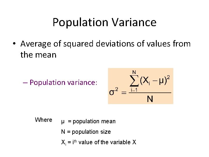
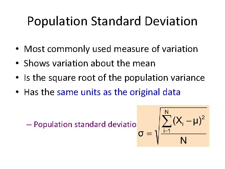
Population Variance • Average of squared deviations of values from the mean – Population variance: Where μ = population mean N = population size Xi = ith value of the variable X

Population Standard Deviation • • Most commonly used measure of variation Shows variation about the mean Is the square root of the population variance Has the same units as the original data – Population standard deviation:

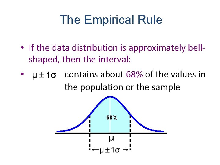
The Empirical Rule • If the data distribution is approximately bellshaped, then the interval: • contains about 68% of the values in the population or the sample 68%

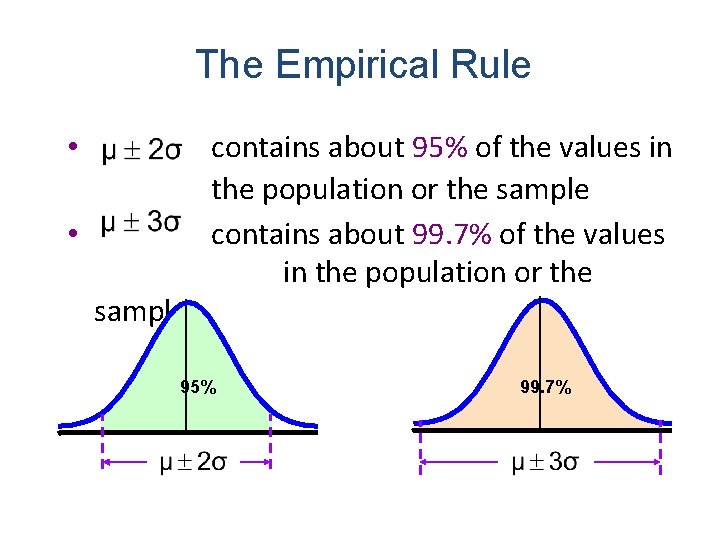
The Empirical Rule • • sample contains about 95% of the values in the population or the sample contains about 99. 7% of the values in the population or the 95% 99. 7%

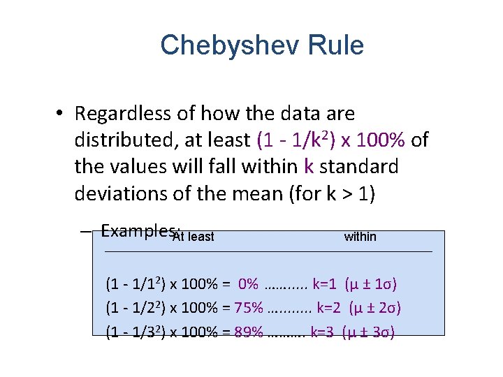
Chebyshev Rule • Regardless of how the data are distributed, at least (1 - 1/k 2) x 100% of the values will fall within k standard deviations of the mean (for k > 1) – Examples: At least within (1 - 1/12) x 100% = 0% ……. . . k=1 (μ ± 1σ) (1 - 1/22) x 100% = 75% …. . . . k=2 (μ ± 2σ) (1 - 1/32) x 100% = 89% ………. k=3 (μ ± 3σ)

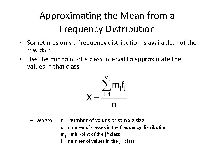
Approximating the Mean from a Frequency Distribution • Sometimes only a frequency distribution is available, not the raw data • Use the midpoint of a class interval to approximate the values in that class – Where n = number of values or sample size c = number of classes in the frequency distribution mj = midpoint of the jth class fj = number of values in the jth class

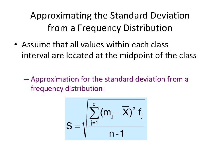
Approximating the Standard Deviation from a Frequency Distribution • Assume that all values within each class interval are located at the midpoint of the class – Approximation for the standard deviation from a frequency distribution:

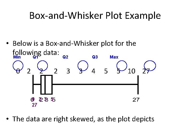
Exploratory Data Analysis • Box-and-Whisker Plot: A Graphical display of data using 5 -number summary: Minimum -- Q 1 -- Median -- Q 3 -- Maximum Example: 25% 25%

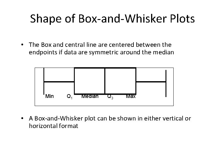
Shape of Box-and-Whisker Plots • The Box and central line are centered between the endpoints if data are symmetric around the median Min Q 1 Median Q 3 Max • A Box-and-Whisker plot can be shown in either vertical or horizontal format

Distribution Shape and Box-and-Whisker Plot Left-Skewed Q 1 Q 2 Q 3 Symmetric Q 1 Q 2 Q 3 Right-Skewed Q 1 Q 2 Q 3

Box-and-Whisker Plot Example • Below is a Box-and-Whisker plot for the following data: Min Q 1 Q 2 Q 3 Max 0 2 2 2 3 3 4 5 5 10 27 0 2 3 5 27 • The data are right skewed, as the plot depicts

Pitfalls in Numerical Descriptive Measures • Data analysis is objective – Should report the summary measures that best meet the assumptions about the data set • Data interpretation is subjective – Should be done in fair, neutral and clear manner

Ethical Considerations Numerical descriptive measures: • Should document both good and bad results • Should be presented in a fair, objective and neutral manner • Should not use inappropriate summary measures to distort facts

Chapter Summary • Described measures of central tendency – Mean, median, mode, geometric mean • Discussed quartiles • Described measures of variation – Range, interquartile range, variance and standard deviation, coefficient of variation, Z-scores • Illustrated shape of distribution – Symmetric, skewed, box-and-whisker plots

Chapter Summary (continued) • Discussed covariance and correlation coefficient • Addressed pitfalls in numerical descriptive measures and ethical considerations