Numerical Descriptive Measures Summary Definitions The central tendency

Numerical Descriptive Measures

Summary Definitions • The central tendency is the extent to which all the data values group around a typical or central value. • The variation is the amount of dispersion, or scattering, of values • The shape is the pattern of the distribution of values from the lowest value to the highest value.

Measures of Central Tendency: The Mean • The arithmetic mean (often just called “mean”) is the most common measure of central tendency Pronounced x-bar The ith value – For a sample of size n: Sample size Observed values

Measures of Central Tendency: The Mean (continued) • The most common measure of central tendency • Mean = sum of values divided by the number of values • Affected by extreme values (outliers) 0 1 2 3 4 5 6 7 8 9 10 Mean = 3 0 1 2 3 4 5 6 7 8 9 Mean = 4 10

Mean for Grouped Data Formula for Mean is given by Where = Mean = Sum of cross products of frequency in each class with midpoint X of each class n = Total number of observations (Total frequency) =

Mean for Grouped Data Example Find the arithmetic mean for the following continuous frequency distribution: Class 0 -1 1 -2 2 -3 3 -4 4 -5 5 -6 Frequency 1 4 8 7 3 2

Solution for the Example Applying the formula = 75. 5/25=3. 02

Mean Class interval f 0 49. 99 78 50 99. 99 123 100 149. 99 187 150 199. 99 82 200 249. 99 51 250 299. 99 47 300 349. 99 13 350 399. 99 9 400 449. 99 6 450 499. 99 4 600

Mean Class interval 0 49. 99 50 99. 99 100 149. 99 150 199. 99 200 249. 99 250 299. 99 300 349. 99 350 399. 99 400 449. 99 450 499. 99 f 78 123 187 82 51 47 13 9 6 4 600 By taking mid values as 25, 75, … 475. Mean: 142. 25

Mean using coding: Class 0 -7 8 -15 16 -23 24 -31 32 -39 40 -47 f 2 6 3 5 2 2 Mean=x 0 + w ((Summation of (u*f)) / n w=numerical width of class interval X 0=value of midpoint assigned code 0

Mean using coding: Class 0 -7 8 -15 16 -23 24 -31 32 -39 40 -47 mid 3. 5 11. 5 19. 5 43. 5 f 2 6 3 5 2 2 Code (u) -2 -1 0 1 2 3 20 Mean=x 0 + w ((Summation of (u*f)) / n = 19. 5+8 (5) / 20 = 21. 5 w=numerical width of class interval X 0=value of midpoint assigned code 0 u*f -4 -6 4 6 5

Weighted mean: Geometric mean: Year 1 2 3 4 5 Interest rate 7% 8 10 12 18 Growth factor 1. 07 1. 08 1. 10 1. 12 1. 18 Saving at the end of year 107. 00 115. 56 168. 00 Mean of growth factor = 1. 07+1. 08+…. . +1. 18)/ 5 = 1. 11, corresponds to 11% rate. 100* (1. 11)*(1. 11)* (1. 11) = 168. 51, correct growth rate should be less than 1. 11. GM = n (1. 07*1. 08*………. *1. 18) 1/n Product of x values = 1. 1093

Measures of Central Tendency: The Median • In an ordered array, the median is the “middle” number (50% above, 50% below) 0 1 2 3 4 5 6 7 8 9 10 Median = 3 • Not affected by extreme values 0 1 2 3 4 5 6 7 8 9 10 Median = 3

Measures of Central Tendency: Locating the Median • The location of the median when the values are in numerical order (smallest to largest): • If the number of values is odd, the median is the middle number • If the number of values is even, the median is the average of the two middle numbers Note that is not the value of the median, only the position of the median in the ranked data

Median for Grouped Data Formula for Median is given by Median = Where L =Lower limit of the median class n = Total number of observations = m = Cumulative frequency preceding the median class f = Frequency of the median class c = Class interval of the median class

Median for Grouped Data Example Find the median for the following continuous frequency distribution: Class Frequency 0 -1 1 1 -2 4 2 -3 8 3 -4 7 4 -5 3 5 -6 2

Solution for the Example Class Frequency Cumulative Frequency 1 5 13 20 23 25 0 -1 1 1 -2 4 2 -3 8 3 -4 7 4 -5 3 5 -6 2 Total 25 Substituting in the formula the relevant values, Median = , we have Median = = 2. 9375

Find median Class interval f 0 49. 99 78 50 99. 99 123 100 149. 99 187 150 199. 99 82 200 249. 99 51 250 299. 99 47 300 349. 99 13 350 399. 99 9 400 449. 99 6 450 499. 99 4 600 300 th = 126. 17 301 st=126. 44

Measures of Central Tendency: The Mode • • • Value that occurs most often Not affected by extreme values Used for either numerical or categorical data There may be no mode There may be several modes 0 1 2 3 4 5 6 7 8 9 10 11 12 13 14 Mode = 9 0 1 2 3 4 5 6 No Mode

Mode for Grouped Data Mode = Where L =Lower limit of the modal class = Frequency preceding the modal class = Frequency succeeding the modal class C = Class Interval of the modal class

Mode for Grouped Data Example: Find the mode for the following continuous frequency distribution: Class Frequency 0 -1 1 1 -2 4 2 -3 8 3 -4 7 4 -5 3 5 -6 2

Solution for the Example Class 0 -1 1 -2 2 -3 3 -4 4 -5 5 -6 Total Frequency 1 4 8 7 3 2 25 Mode = L = 2 = 8 -4 = 4 = 8 -7 = 1 C = 1 Hence Mode = = 2. 8

Measures of Central Tendency: Which Measure to Choose? The mean is generally used, unless extreme values (outliers) exist. The median is often used, since the median is not sensitive to extreme values. For example, median home prices may be reported for a region; it is less sensitive to outliers. In some situations it makes sense to report both the mean and the median.

Measures of Central Tendency: Summary Central Tendency Arithmetic Mean Median Middle value in the ordered array Mode Most frequently observed value

Measures of Variation Range Variance Standard Deviation Coefficient of Variation Measures of variation give information on the spread or variability or dispersion of the data values. Same center, different variation

Measures of Variation: The Range § Simplest measure of variation § Difference between the largest and the smallest values: Range = Xlargest – Xsmallest Example: 0 1 2 3 4 5 6 7 8 9 10 11 12 13 14 Range = 14 - 1 = 13

Measures of Variation: Why The Range Can Be Misleading § Ignores the way in which data are distributed 7 8 9 10 11 12 7 8 Range = 12 - 7 = 5 9 10 11 Range = 12 - 7 = 5 § Sensitive to outliers 1, 1, 1, 2, 2, 3, 3, 4, 5 Range = 5 - 1 = 4 1, 1, 1, 2, 2, 3, 3, 4, 120 Range = 120 - 1 = 119 12

Interfractile range: Median is. 5 fractile. First third 863 903 957 1041 Second third 1138 1204 1354 1624 1/3 fractile Last third 1698 1745 1802 1883 2/3 fractile If we divide data in? ? ? ? deciles , quartile and percentile Interquartile range: Q 3 -Q 1

Measures of Variation: The Variance • Average (approximately) of squared deviations of values from the mean – Sample variance: Where = arithmetic mean n = sample size Xi = ith value of the variable X

Measures of Variation: The Standard Deviation • • Most commonly used measure of variation Shows variation about the mean Is the square root of the variance Has the same units as the original data – Sample standard deviation:

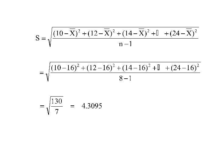
Measures of Variation: The Standard Deviation Steps for Computing Standard Deviation 1. 2. 3. 4. 5. Compute the difference between each value and the mean. Square each difference. Add the squared differences. Divide this total by n-1 to get the sample variance. Take the square root of the sample variance to get the sample standard deviation.

Measures of Variation: Sample Standard Deviation: Calculation Example Sample Data (Xi) : 10 12 14 15 17 18 18 24 n = 8 Mean = X = 16

Class Frequency 700 -799 4 800 -899 7 900 8 1000 10 1100 12 1200 17 1300 13 1400 10 1500 9 1600 7 1700 2 1800 -1899 1 Find S. D.

Measures of Variation: Comparing Standard Deviations Data A Mean = 15. 5 11 12 13 14 15 16 17 18 19 20 Data B 11 12 21 S = 3. 338 Mean = 15. 5 13 14 15 16 17 18 19 20 21 Data C S = 0. 926 Mean = 15. 5 S = 4. 570 11 12 13 14 15 16 17 18 19 20 21

Measures of Variation: Comparing Standard Deviations Smaller standard deviation Larger standard deviation

Standard Deviation for Grouped Data-Example Frequency Distribution of Return on Investment of Mutual Funds Return on Number of Investment Mutual Funds 5 -10 10 -15 15 -20 20 -25 25 -30 Total 10 12 16 14 8 60

Solution for the Example

Solution for the Example From the spreadsheet of Microsoft Excel in the previous slide, it is easy to see Mean = =1040/60=17. 333(cell F 10), Standard Deviation = S = = 6. 44 (Cell H 12)

Measures of Variation: Summary Characteristics § The more the data are spread out, the greater the range, variance, and standard deviation. § The more the data are concentrated, the smaller the range, variance, and standard deviation. § If the values are all the same (no variation), all these measures will be zero. § None of these measures are ever negative.

Measures of Variation: The Coefficient of Variation • Measures relative variation • Always in percentage (%) • Shows variation relative to mean • Can be used to compare the variability of two or more sets of data measured in different units

Measures of Variation: Comparing Coefficients of Variation • Stock A: – Average price last year = $50 – Standard deviation = $5 • Stock B: – Average price last year = $100 – Standard deviation = $5

Measures of Variation: Comparing Coefficients of Variation • Stock A: – Average price last year = $50 – Standard deviation = $5 • Stock B: – Average price last year = $100 – Standard deviation = $5 Both stocks have the same standard deviation, but stock B is less variable relative to its price

Shape of a Distribution • Describes how data are distributed • Measures of shape – Symmetric or skewed Left-Skewed(Negative)) Mean < Median Symmetric Mean = Median Right-Skewed (Positive) Median < Mean