Introduction to Statistics Measures of Central Tendency Two

Introduction to Statistics Measures of Central Tendency

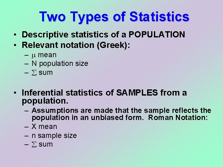
Two Types of Statistics • Descriptive statistics of a POPULATION • Relevant notation (Greek): – mean – N population size – sum • Inferential statistics of SAMPLES from a population. – Assumptions are made that the sample reflects the population in an unbiased form. Roman Notation: – X mean – n sample size – sum

• Be careful though because you may want to use inferential statistics even when you are dealing with a whole population. • Measurement error or missing data may mean that if we treated a population as complete that we may have inefficient estimates. – It depends on the type of data and project. – Example of Democratic Peace.

• Also, be careful about the phrase “descriptive statistics”. It is used generically in place of measures of central tendency and dispersion for inferential statistics. • Another name is “summary statistics”, which are univariate: – Mean, Median, Mode, Range, Standard Deviation, Variance, Min, Max, etc.

Measures of Central Tendency • These measures tap into the average distribution of a set of scores or values in the data. – Mean – Median – Mode

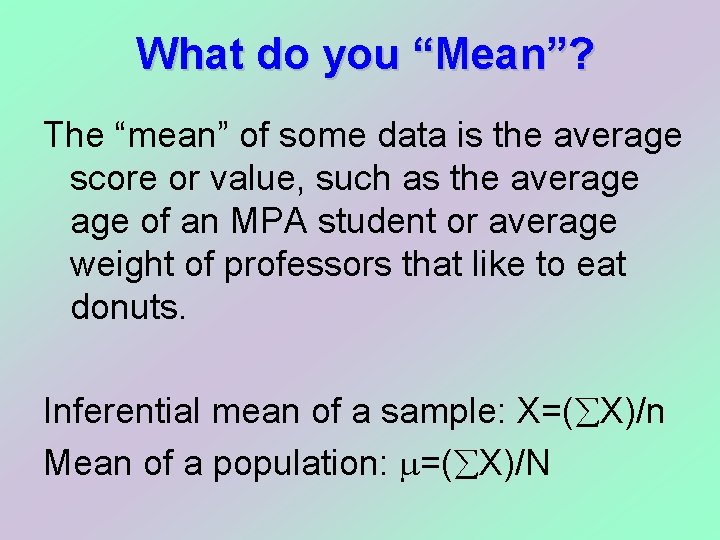
What do you “Mean”? The “mean” of some data is the average score or value, such as the average of an MPA student or average weight of professors that like to eat donuts. Inferential mean of a sample: X=( X)/n Mean of a population: =( X)/N

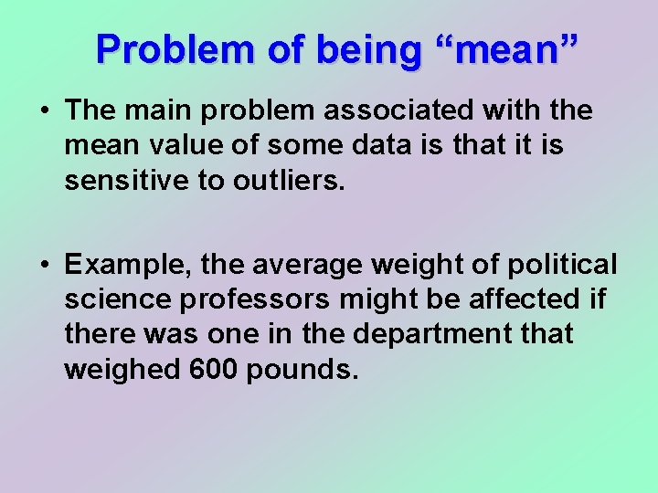
Problem of being “mean” • The main problem associated with the mean value of some data is that it is sensitive to outliers. • Example, the average weight of political science professors might be affected if there was one in the department that weighed 600 pounds.

Donut-Eating Professors Professor Weight Schmuggles 165 Bopsey 213 Pallitto 189 410 Homer 187 610 Schnickerson 165 Levin 148 Honkey-Doorey 251 Zingers 308 Boehmer 151 Queenie 132 Googles-Boop 199 Calzone 227 194. 6 248. 3

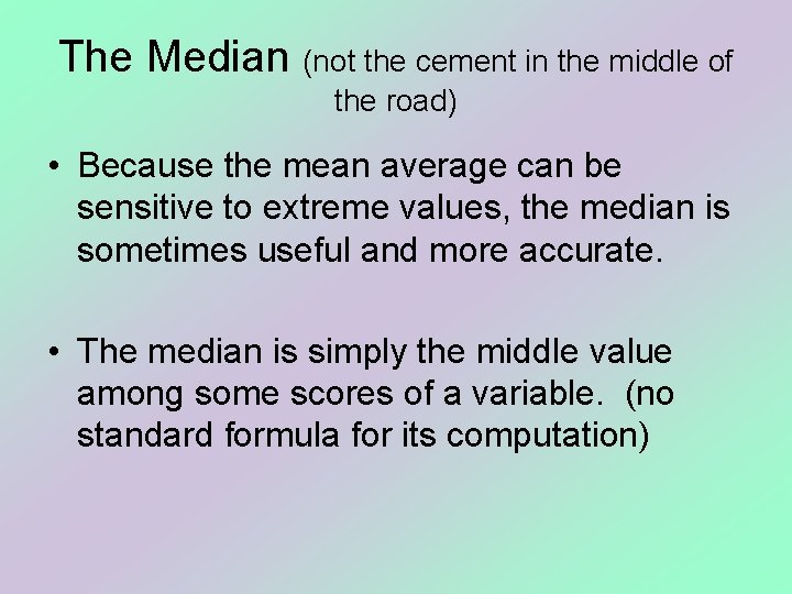
The Median (not the cement in the middle of the road) • Because the mean average can be sensitive to extreme values, the median is sometimes useful and more accurate. • The median is simply the middle value among some scores of a variable. (no standard formula for its computation)

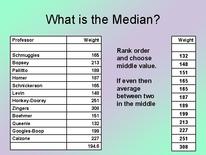
What is the Median? Professor Weight Rank order and choose middle value. Schmuggles 165 Bopsey 213 Pallitto 189 Homer 187 Schnickerson 165 Levin 148 Honkey-Doorey 251 Zingers 308 Boehmer 151 199 Queenie 132 213 Googles-Boop 199 227 Calzone 227 251 194. 6 308 132 148 151 If even then average between two in the middle 165 187 189

Percentiles • If we know the median, then we can go up or down and rank the data as being above or below certain thresholds. • You may be familiar with standardized tests. 90 th percentile, your score was higher than 90% of the rest of the sample.

The Mode (hold the pie and the ala) (What does ‘ala’ taste like anyway? ? ) • The most frequent response or value for a variable. • Multiple modes are possible: bimodal or multimodal.

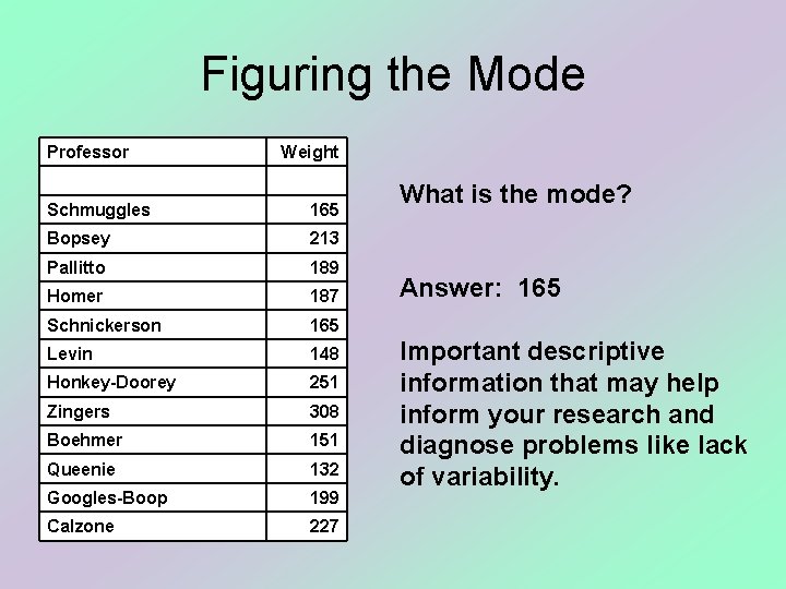
Figuring the Mode Professor Weight Schmuggles 165 Bopsey 213 Pallitto 189 Homer 187 Schnickerson 165 Levin 148 Honkey-Doorey 251 Zingers 308 Boehmer 151 Queenie 132 Googles-Boop 199 Calzone 227 What is the mode? Answer: 165 Important descriptive information that may help inform your research and diagnose problems like lack of variability.

Measures of Dispersion (not something you cast…) • Measures of dispersion tell us about variability in the data. Also univariate. • Basic question: how much do values differ for a variable from the min to max, and distance among scores in between. We use: – Range – Standard Deviation – Variance

• Remember that we said in order to glean information from data, i. e. to make an inference, we need to see variability in our variables. • Measures of dispersion give us information about how much our variables vary from the mean, because if they don’t it makes it difficult infer anything from the data. Dispersion is also known as the spread or range of variability.

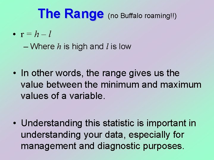
The Range (no Buffalo roaming!!) • r=h–l – Where h is high and l is low • In other words, the range gives us the value between the minimum and maximum values of a variable. • Understanding this statistic is important in understanding your data, especially for management and diagnostic purposes.

The Standard Deviation • A standardized measure of distance from the mean. • Very useful and something you do read about when making predictions or other statements about the data.

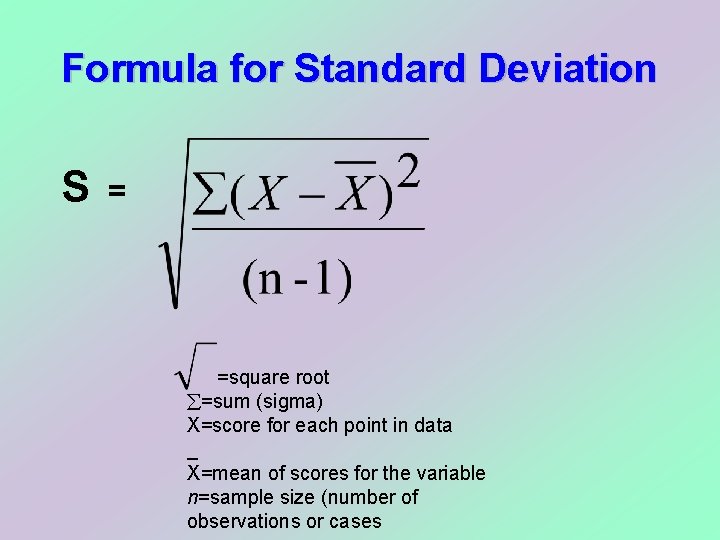
Formula for Standard Deviation S = =square root =sum (sigma) X=score for each point in data _ X=mean of scores for the variable n=sample size (number of observations or cases

We can see that the Standard Deviation equals 165. 2 pounds. The weight of Zinger is still likely skewing this calculation (indirectly through the mean).

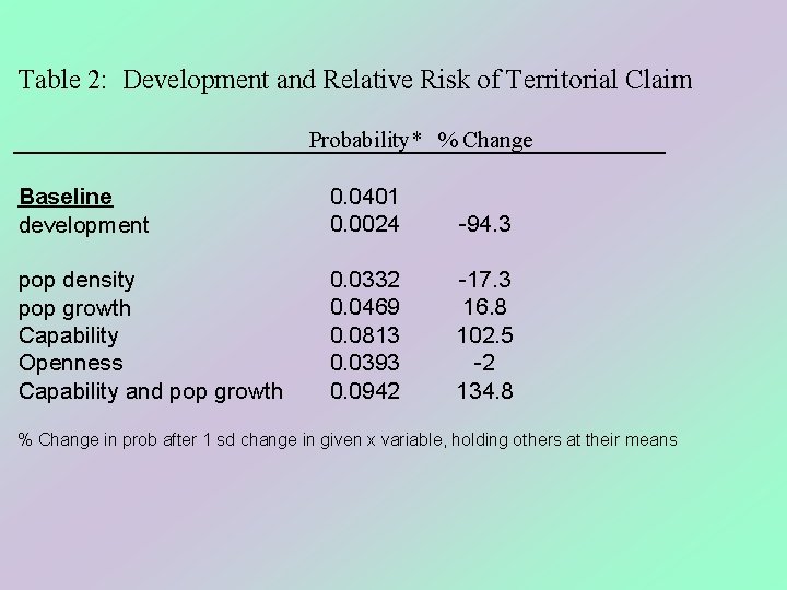
Example of S in use • Boehmer- Sobek paper. – One standard deviation increase in the value of X variable increases the Probability of Y occurring by some amount.

Table 2: Development and Relative Risk of Territorial Claim Probability* % Change Baseline development 0. 0401 0. 0024 -94. 3 pop density pop growth Capability Openness Capability and pop growth 0. 0332 0. 0469 0. 0813 0. 0393 0. 0942 -17. 3 16. 8 102. 5 -2 134. 8 % Change in prob after 1 sd change in given x variable, holding others at their means

Let’s go to computers! • Type in data in the Excel sheet.

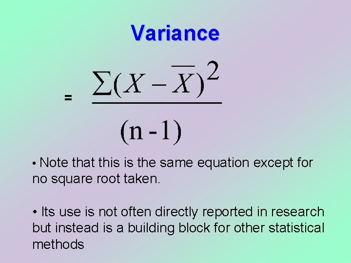
Variance = • Note that this is the same equation except for no square root taken. • Its use is not often directly reported in research but instead is a building block for other statistical methods

Organizing and Graphing Data

Goal of Graphing? 1. Presentation of Descriptive Statistics 2. Presentation of Evidence 3. Some people understand subject matter better with visual aids 4. Provide a sense of the underlying data generating process (scatterplots)

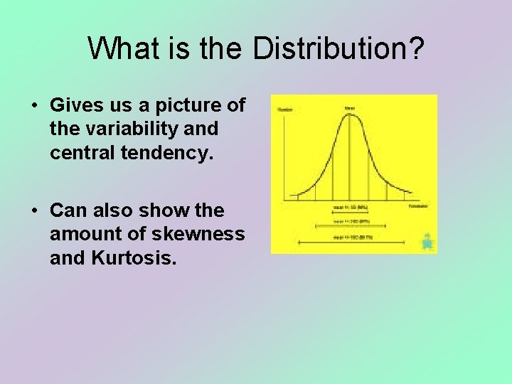
What is the Distribution? • Gives us a picture of the variability and central tendency. • Can also show the amount of skewness and Kurtosis.

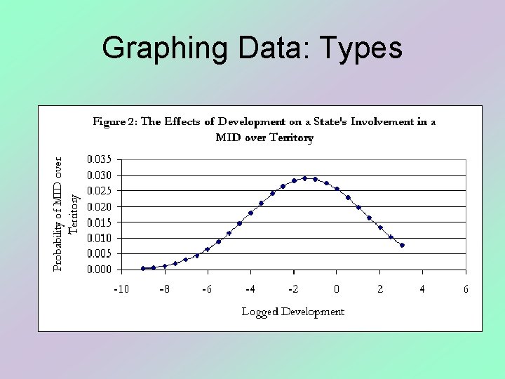
Graphing Data: Types

Creating Frequencies • We create frequencies by sorting data by value or category and then summing the cases that fall into those values. • How often do certain scores occur? This is a basic descriptive data question.

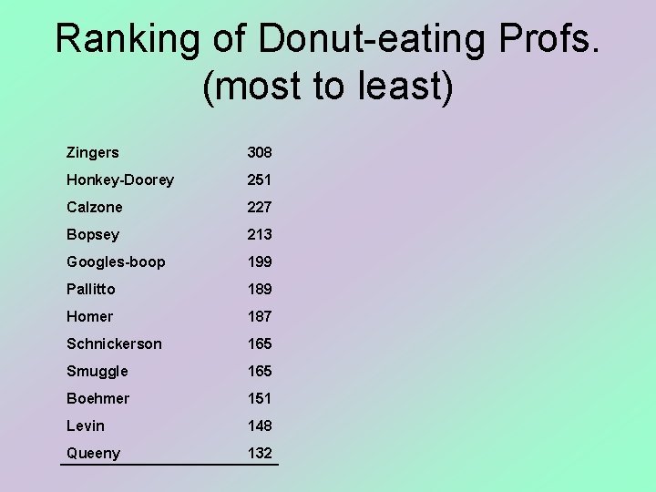
Ranking of Donut-eating Profs. (most to least) Zingers 308 Honkey-Doorey 251 Calzone 227 Bopsey 213 Googles-boop 199 Pallitto 189 Homer 187 Schnickerson 165 Smuggle 165 Boehmer 151 Levin 148 Queeny 132

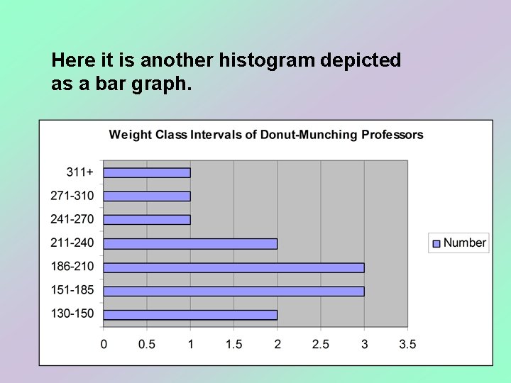
Here we have placed the Professors into weight classes and depict with a histogram in columns.

Here it is another histogram depicted as a bar graph.

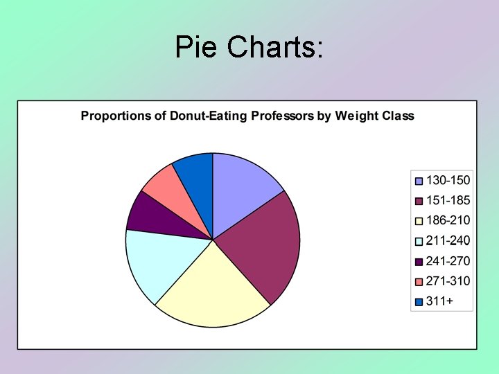
Pie Charts:

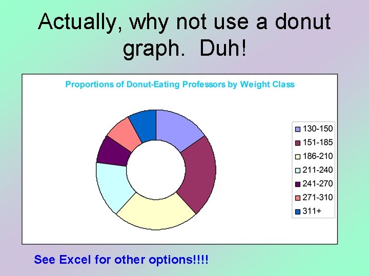
Actually, why not use a donut graph. Duh! See Excel for other options!!!!

Line Graphs: A Time Series

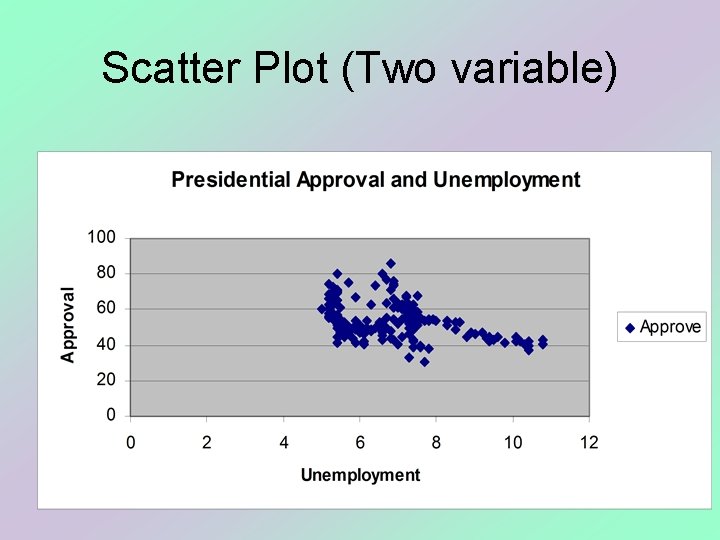
Scatter Plot (Two variable)