Repeated Measures Design Group 5 Jian Wang Xi

Repeated Measures Design Group 5: Jian Wang, Xi Zhang, Yan Cao, Qichao Sun, Jixiang Zhang, Zishan Chen, Xing Peng, Xiao Liu

Introduction to repeated measures design Jian Wang

Review of paired sample t-test • A paired sample t-test is used to determine whethere is a significant difference between the average values of the same measurement made under two different conditions. The usual null hypothesis is that the difference in the mean values is zero. • －－－repeated measures design is actually an extension of paired sample t－test or we can say paired t test is a special case in the repeated measures design(which involved only two related measures)

What is repeated measures design A repeated-measures design is one in which multiple, or repeated, measurements are made on each experimental unit under different conditions.

Simple Example • Students were asked to rate their stress on a 50 point scale in the week before, the week of, or the week after their midterm exam.

Advantages－why use repeated measures design • Require fewer participants－－This design is economical because each member is measured under all conditions. • Eliminating individual differences－－ collecting data from the same participants under repeated conditions so it reduces individual difference and the test becomes more powerful. • Longitudinal analysis—Repeated measure design is especially good for researchers to monitor how participants change over time.

Disadvantage • Carry－over effect：an effect that “carries over” from one experimental condition to another when subjects perform in more than one condition.

One-Way Repeated Measures ANOVA

Compared with One-Way ANOVA • One-Way ANOVA: we look at differences between different samples that come from different groups within a single factor. – That is, 1 factor, k levels k separate groups are compared. • One-Way RM ANOVA: we can answer the same question looking at just 1 sample that is exposed to different manipulations within a factor. – That is, 1 factor, k levels only 1 group is compared across k conditions.

• For normal One-Way ANOVA, we use a different groups to test these a levels. So the observations between treatments are independent. • But for One-way RM ANOVA, we use only one group to test these a levels. So the observations between treatments are dependent.

Compared with One-Way ANOVA • MODEL: Yij= μi+εij μi: the mean of the ith treatment. εij: the random error which follows N(0, σow 2)

Compared with One-Way ANOVA • MODEL: Yij= μi+Bj+ε’ij μ i: the mean of the ith treatment. Bj: a parameter associated with jth subject which follows N(0, σB 2). ε’ij: the random error which follows N(0, σRMOW 2) and is independent with Bj

Compared with One-Way ANOVA • One-Way ANOVA TABLE Source DF Treatment a-1 Error N-a Total N-1 SS MS σOW 2

Compared with One-Way ANOVA • One-Way RM ANOVA TABLE Source DF Treatment a-1 Subject n-1 Error (a-1)(n-1) Total N-1 SS MS σRMOW 2

Compared with One-Way ANOVA • Partition of Sum of Square Standard ANOVA SSTOTAL SStreatment Repeated Measures ANOVA SSerror SSbetween subject SSwithin subject SStreatment SSerror

Compared with paired sample t-test • Example (2 treatments)

Compared with paired sample t-test • Hypothesis • T-TEST

Compared with paired sample t-test • T-TEST Since So

Compared with paired sample t-test • F-TEST

Compared with paired sample t-test • F-TEST

Compared with paired sample t-test • The paired sample t-test is just the One-way Repeated measures design. • Repeated measures design are considered an extension of the paired sample t-test when comparisons between more than two repeated measures are needed.

one-way repeated measure ANOVA Repeated measures one-way ANOVA compares the means of two or more matched groups. When to use? repeated measures ANOVA is used when all members of a random sample are measured under a number of different conditions

one-way repeated measure ANOVA Model Yij = μi +Sj+εij μi = The fixed effect. Sj= The random effect of subject j. εij = The random error independent of Sj.

one-way repeated measure ANOVA • Repeated Measures ANOVA Table SS Df Between a-1 Within N-a -Subjects s-1 -Error Total N-1 MS F

one-way repeated measure ANOVA Example: • We have four drugs (1, 2, 3 and 4) that relieve pain. Each subject is given each of the four drugs. The subject’s pain tolerance is then measured. Enough time is allowed to pass between successive drug administrations so that we can be sure there’s no residual effect from the previous drug. Are there any difference between the four drugs using significant level �� =0. 05? data from the pain experiment: SUBJECT DRUG 1 DRUG 2 DRUG 3 DRUG 41 1 5 9 6 11 2 7 12 8 9 3 11 12 10 14 4 3 8 5 8 �� 0: �� 1=�� 2=�� 3=�� 4 �� : �� ������ �� 0 ����

one-way repeated measure ANOVA SUBJECT DRUG 1 DRUG 2 DRUG 3 DRUG 41 1 5 9 6 11 2 7 12 8 9 3 11 12 10 14 4 3 8 5 8

one-way repeated measure ANOVA SUBJECT DRUG 1 DRUG 2 DRUG 3 DRUG 4 Y. j 1 5 9 6 11 7. 75 2 7 12 8 9 9 3 11 12 10 14 11. 75 4 3 8 5 8 6 Yi. 6. 5 10. 25 7. 25 10. 5 Y. . =8. 625 SS Treatment =R× ∑(Yi. − Y. . )2= 4 × 12. 5625=50. 25 SS Subject = I × ∑(Y. j − Y. . )2= 4 × 17. 5625 = 70. 25 SS Total = ∑ ∑(Yij − Y. . ) 2=133. 75 SS Error = ∑ ∑(Yij − Yi. − Y. j + Y. . )2 = SS Total − SS Treatment − SS Subject = 13. 25

one-way repeated measure ANOVA SUBJECT DRUG 1 DRUG 2 DRUG 3 DRUG 4 Y. j 1 5 9 6 11 7. 75 2 7 12 8 9 9 3 11 12 10 14 11. 75 4 3 8 5 8 6 Yi. 6. 5 10. 25 7. 25 10. 5 Y. . =8. 625

one-way repeated measure ANOVA SAS Code data pain; input subj@; do drug = 1 to 4 ; input pain @; output; end; datalines; 1 5 9 6 11 2 7 12 8 9 3 11 12 10 14 4 3 8 5 8 ; proc anova data = pain; title'one-way Repeatede Measures ANOVA'; class subj drug; model pain = subj drug; means drug/duncan; run;

one-way repeated measure ANOVA • SAS output:

Two –factor experiments with a repeated measure on one factor Qichao Sun

Why do we need the two-factor ANOVA with a repeated measure on one factor? 1）mean scores in each treatment group change over two or more time points. 2）under two or more different conditions, there are differences in mean scores in one treatment group.

Example • To investigate the effect of the drug, which needs several hours to have effects on patients. There are four groups with different dose of drug. Obviously, we cannot be sure if the effects are caused by the dose (maybe time has an effect). So we add the other factor ‘time’, and measure the observation before and after the treatment. Control Group (placebo) Treatment Group 2 ( 1. 00 mg) Treatment Group 3 ( 1. 25 mg) Treatment Group 4 ( 1. 50 mg) Subject Before After 1 80 83 2 85 86 3 83 88 4 82 94 5 87 93 6 84 98 7 85 102 8 87 98 9 83 97 10 86 107 11 82 103 12 88 106

• In this example, we have two factors, the dose of the drug and the time. Here we call the dose Factor A and the time Factor B. And we use the same subjects in one level of Factor A before and after the treatment. So Factor B ‘time’ is the factor with repeated measure. • This setting is two factor ANOVA with repeated measure on one factor. The appropriate error term for the test of the dose is subject|dose. The appropriate error term for time and time*dose is time*subject|dose (which is the residual error since we do not include the term in the model).

Model •

Hypothesis •

ANOVA Table Source Factor A Dose Factor B Time AB Interaction Time*Dose Subjects within A DF SS I-1=3 SSA MS SSA/(I-1) J-1=1 SSB/(J-1) (I-1)(J-1)=3 SSAB/(I-1)(J-1) I(K-1)=8 SSWA/I(K-1) I(J-1)(K-1)=8 IJK-1 SSE SST SSE/I(J-1)(K-1) subject|d ose Error Total , where I=4, J=2, K=3 F

Sum of Square •

Test statistic •

The SAS code is following. data drug; input subj dose $ before after; datalines; 1 C 80 83 2 C 85 86 3 C 83 88 4 T 2 82 94 5 T 2 87 93 6 T 2 84 98 7 T 3 85 102 8 T 3 87 98 9 T 3 83 97 10 T 4 86 107 11 T 4 82 103 12 T 4 88 106 ; proc anova data= drug; class dose; model before after= dose / nouni; repeated time 2 (0 1); means dose; run;

SAS Output for repeated statement MANOVA Test Criteria and Exact F Statistics for the Hypothesis of no time Effect H = Anova SSCP Matrix for time E = Error SSCP Matrix S=1 M=-0. 5 N=3 Statistic Value F Value Num DF Den DF Pr > F Wilks' Lambda 0. 03764883 204. 49 1 8 <. 0001 Pillai's Trace 0. 96235117 204. 49 1 8 <. 0001 Hotelling-Lawley Trace 25. 56125000 204. 49 1 8 <. 0001 Roy's Greatest Root 25. 56125000 204. 49 1 8 <. 0001 MANOVA Test Criteria and Exact F Statistics for the Hypothesis of no time*dose Effect H = Anova SSCP Matrix for time*dose E = Error SSCP Matrix S=1 M=0. 5 N=3 Statistic Value F Value Num DF Den DF Pr > F Wilks' Lambda 0. 12847278 18. 09 3 8 0. 0006 Pillai's Trace 0. 87152722 18. 09 3 8 0. 0006 Hotelling-Lawley Trace 6. 78375000 18. 09 3 8 0. 0006 Roy's Greatest Root 6. 78375000 18. 09 3 8 0. 0006

How to choose Multivariate statistics? • The output shows that there are four F statistics: • Wilks’ Lambda • Pillai’s Trace • Hotelling- Lawley Trace • Roy’s Greatest Root • If there are only very small differences among the P-values, we can either of them or choose Wilks’ Lambda which is often appropriate. • If not, find consultant.

The ANOVA Procedure Repeated Measures Analysis of Variance Tests of Hypotheses for Between Subjects Effects Source DF Anova SS Mean Square F Value Pr > F dose 3 397. 4583333 132. 4861111 15. 59 0. 0011 Error 8 68. 0000000 8. 5000000 The ANOVA Procedure Repeated Measures Analysis of Variance Univariate Tests of Hypotheses for Within Subject Effects Source DF Anova SS Mean Square F Value Pr > F time 1 852. 0416667 204. 49 <. 0001 time*dose 3 226. 1250000 75. 3750000 18. 09 0. 0006 Error(time) 8 33. 3333333 4. 1666667

The Other method without using repeated statement • Two-factor ANOVA without using the REPEATED statement • SAS code: data twoway; set drug; /* ‘SET’ causes observations to be read from the original data set*/ length time $ 7; /*set the length of variable ‘Time’*/ time = ‘before’; /*creat a new variable ‘Time’ and set the value of Time to ‘before’*/ score =before; /*creat a new variable ‘Score’ equl to the before value*/ output; /*the first observation in data set TWOWAY*/ time = ‘after’; score = after; output; keep subj dose time score; run;

proc anova data=twoway; class subj dose time; model score = dose subj(dose) time dose*time*subj(dose); /*In the model statement, all sources of variation are included, so SSE will be 0. */ means dose|time; test H=dose E=subj(dose); test H=time dose*time E=time*subj(dose); /*the error term for dose is subj(dose), and the error term for time and dose*time is time*subj(dose). */ run;

Output for the method without repeated statement Class Level Information Class Levels Values subj 12 1 2 3 4 5 6 7 8 9 10 11 12 dose 4 C T 2 T 3 T 4 time 2 after before Source DF Sum of Squares Mean Square F Value Pr > F Model 23 1576. 958333 68. 563406 . . Error 0 0. 000000 . 1576. 958333 Corrected 23 Total Model statement contains all sources of variation about the grand mean. So SSE is 0. Source DF Anova SS Mean Square F Value Pr > F dose 3 397. 4583333 132. 4861111 . . subj(dose) 8 68. 0000000 8. 5000000 . . time 1 852. 0416667 . . dose*time 3 226. 1250000 75. 3750000 . . 33. 3333333 4. 1666667 . . subj*time(dose) 8

Level of dose N C score Mean Std Dev 6 84. 1666667 2. 7868740 T 2 6 89. 6666667 6. 2822501 T 3 6 92. 0000000 7. 9498428 T 4 6 95. 3333333 11. 2011904 Level of group Level of time N C post C score Mean Std Dev 3 85. 6666667 2. 51661148 pre 3 82. 6666667 2. 51661148 T post 3 95. 0000000 2. 64575131 T pre 3 84. 3333333 2. 51661148 Tests of Hypotheses Using the Anova MS for subj(dose) as an Error Term Source DF Anova SS Mean Square F Value Pr > F dose 3 397. 4583333 132. 4861111 15. 59 0. 0011 Tests of Hypotheses Using the Anova MS for subj*time(dose) as an Error Term Source DF Anova SS Mean Square F Value Pr > F time 1 852. 0416667 204. 49 <. 0001 dose*time 3 226. 1250000 75. 3750000 18. 09 0. 0006

Two-Factor ANOVA with Repeated Measures on both Factors Jixiang Zhang 2/28/2021

The model is This design is similar to the previous design except that each subject is measured under all levels of both factor.

ANOVA TABLE Source DF SS MS F Subjects n-1 SSS/I-1 MSS/MSE Factor A a-1 SSA/(a-1) MSA/MSA*S ～ F(a-1), (n 1)(a-1) Factor B b-1 SSB/(b-1) MSB/MSB*S ～ F(b-1), (n 1)(b-1) SSAB/((a-1)(b- MSAB/MSE～F(a-1)(b-1), (n 1)) 1)(a-1)(b-1) AB Interaction (a-1)(b-1) SSAB A*Subjects (n-1)(a-1) SSA*S SSWA/((n-1)a) SSA*S/MSE F(a-1)(n-1), (n-1)(a-1)(b-1) B*Subjects (n-1)(b-1) SSB*S SSWB/((n-1)b) SSA*S/MSE F(n-1)(b-1), (n-1)(a-1)(b-1) Error Total (n-a)(a-1)(b- SSE 1) nab-1 SST SSE/((n-1)(a 1)(b-1))

Example: A group of subjects is treated in the morning and afternoon of two different days. On one of the days, the subjects receive a strong sleeping aid the night before the experiment is to be conducted; on the other, a placebo.

A diagram of the experiment Treatment Time A. M. P. M Control Subject 1 2 3 Drug Reaction Subject 65 1 72 2 90 3 55 1 64 2 80 3 Reaction 70 78 97 60 68 85

• We would like to see if the drug had any effect on the reaction time and if the effect was the same for the whole day. • We can use the AM/PM measurements on the control day as a comparison for the AM/PM changes on the drug days. • Since each subject is measured under all levels of treatment(PLACEBO or DRUG) and TIME(AM/PM), we can treat this experiment as a SUBJ by TREATMENT by TIME factorial design. However, we must specify the error terms to test our hypotheses.

• In any design where all factors are repeated, such as this one, we can treat the SUBJ variable as being crossed by all other factors. • However, by including the SUBJ term in our model, the error term will be zero. • The error terms to test each hypothesis are simpler to remember: For factor X, the error term is SUBJ*X.

SAS CODE data repeat; proc anova data=repeat; input react 1 -react 4; model react 1 -react 4= datalines; 65 70 55 60 72 78 64 68 /nouni; repeated time 2, treat 2 90 97 80 85 /nom; ; run; Run;

A portion of output from SAS

Interpretation • According to the observed p-values, The drug increase reaction time(F=256. 00, P=. 0039) • Reaction time is longer in the morning compared to the afternoon(F=300. 00, P=. 0033) • The interaction of treat and time is not significant(F=4. 00, P=0. 1835)

Three-factor Experiments with a repeated measure Zishan Chen

ANOVA Table Source d. f SS MS Factor A a-1 SSA MSA=SSA/(a-1) Factor B b-1 SSB MSB=SSB/(b-1) Factor C(repeated) c-1 SSC MSC=SSC/(c-1) Subjects(within AB) ab(i-1) SSWAB MSWAB= SSWAB/(ab(i-1)) AB interaction (a-1)(b-1) SSAB MSAB =SSAB/(a-1)(b-1) AC interaction (a-1)(c-1) SSAC MSAC = SSAC/(a-1)(c-1) BC interaction (b-1)(c-1) SSBC MSBC = SSBC/(b-1)(c-1) ABC interaction (a-1)(b-1) (c 1) SSABC MSABC = SSABC/(a-1)(b-1) (c-1) Error ab(c-1)(i-1) SSE MSE = SSE/ab(c-1)(i-1) Total Abci-1 SST

Example • There is a marketing experiment. • Male and female subjects are offered one of three different brands of coffee: A, B, C. • Each brand is tasted twice. After breakfast and After dinner. • The preference of each brand is measured on a scale from 1 to 10

The results of the experiment Bran d A SUB J GEN DER B C Brkfs Dinne SUB Brkfst Dinne r J r M 1 7 8 7 4 6 13 8 9 2 6 7 8 3 5 14 6 9 3 6 8 9 3 5 15 5 8 4 5 7 10 3 4 16 6 9 5 4 7 11 4 4 17 6 9 6 4 6 12 2 3 18 7 8 F BRAND and GENDER are crossed MEAL: Repeated Measure Factor

The SAS code • • • • • • data coffee; input subj brand $ gender $ score_B score_D; datalines; 1 A M 7 8 2 A M 6 7 3 A M 6 8 4 A F 5 7 5 A F 4 7 6 A F 4 6 7 B M 4 6 8 B M 3 5 9 B M 3 5 10 B F 3 4 11 B F 4 4 12 B F 2 3 13 C M 8 9 14 C M 6 9 15 C M 5 8 16 C F 6 9 17 C F 6 9 18 C F 7 8 ;

THE SAS CODE “nouni” means that we do not want univariate statistics for score_b and score_d proc anova data=coffee; title "coffee study"; class brand gender; model score_b score_d = brand | gender / nouni; repeated meal; means brand | gender; run; “brand | gender” meams brand + gender+brand *gender

Selected output 1

Selected output 2

Selected output 3

Selected output 4

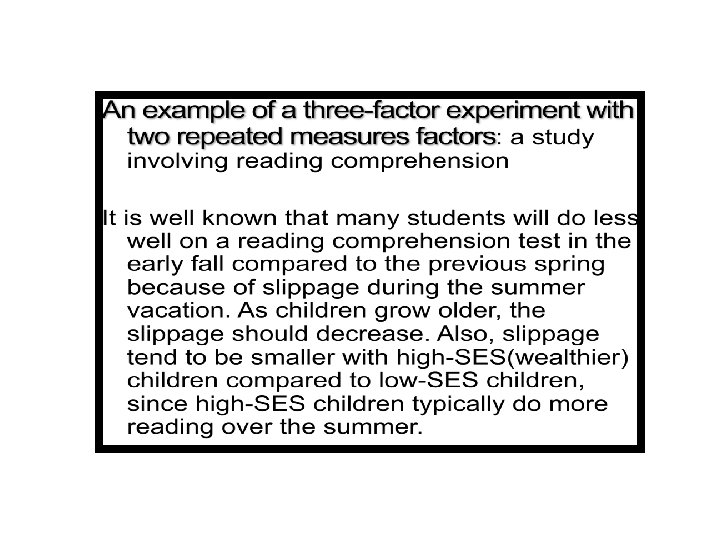
Three-Factor Experiments With Repeated Measures on Two Factors

To test these ideas, the following experiment was devised: • A group of high- and low-SES children is selected for the experiment. Their reading comprehension is tested each spring and fall for three consecutive years. A Diagram of the design is shown below:

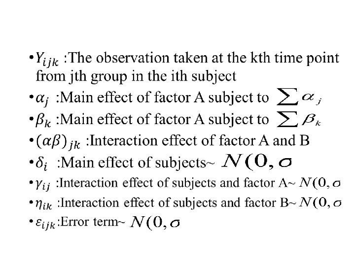
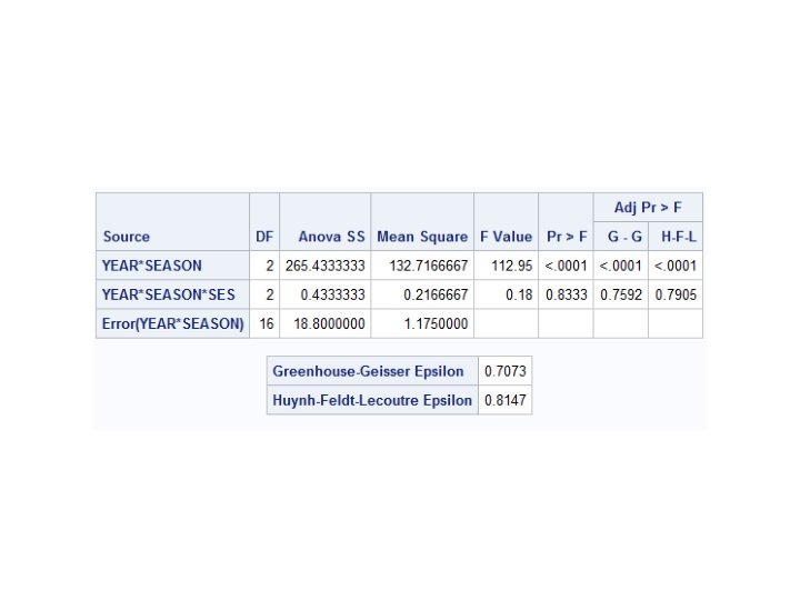
Notice that each subject is measured each spring and fall of each year so that the variables SEASON and YEAR are both repeated measures factors. To analyze this experiment, we will use the SAS program: the REPEATED statement of PROC ANOVA: • DATA READ • INPUT SUBJ SES $ READ 1 READ 2 READ 3 READ 4 READ 5 READ 6; • LABEL READ 1 = ' SPRING YR 1 ' • READ 2 = ' FALL YR 1 ' • READ 3 = ' SPRING YR 2 ' • READ 4 = ' FALL YR 2 ' • READ 5 = ' SPRING YR 3 ' • READ 6 = ' FALL YR 3 ';

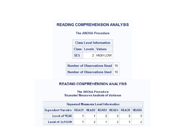
DATALINES; 1 HIGH 61 50 60 55 59 62 2 HIGH 64 55 62 57 63 63 3 HIGH 59 49 58 52 60 58 4 HIGH 63 59 65 64 67 70 5 HIGH 62 51 61 56 60 63 6 LOW 57 42 56 46 54 50 7 LOW 61 47 58 48 59 55 8 LOW 55 40 55 46 57 52 9 LOW 59 44 61 50 63 60 10 LOW 58 44 56 49 55 49 ; PROC ANOVA DATA=READ; TITLE "READING COMPREHENSION ANALYSIS"; CLASS SES; MODEL READ 1 -READ 6 = SES / NOUNI; REPEATED YEAR 3, SEASON 2; MEANS SES; RUN;

• Since the REPEATED statement is confusing when we have more than one repeated factor, it is important for you to know how to determine the order of the factor names. Look at the REPEATED statement in this example: REPEATED YEAR 3, SEASON 2; This statement instructs the ANOVA procedure to choose the first level of YEAR(1), then loop through two levels of SEASON(SPRING FALL), then return to the next level of YEAR(2), followed by two levels of SEASON, etc.

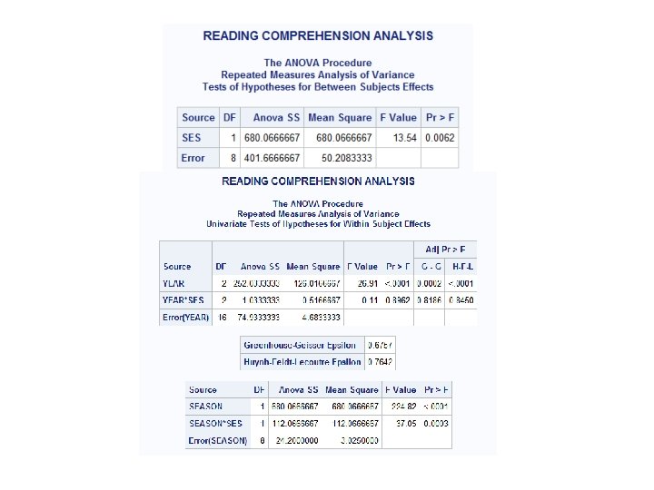
• High-SES student have higher reading comprehension scores than low-SES students (F=13. 54, p=0. 0062). • Reading comprehension increases with each year (F=26. 91, p=0. 0001). • Students had higher reading comprehension scores in the spring compared to the following fall (F=224. 82, p=0. 0001) • The "slippage" was greater for the low-SES students (there was a significant SES*SEASON interaction [F=37. 05, p=0. 0003}). • "Slippage" decreases as the students get older (YEAR*SEASON is significant [F=112. 95, p=0. 0001]).

Independent Measures Design vs. Repeated Measures Design in ANOVA

• Experimental design is a method of assigning observations to different groups in an experiment. • Independent-measures design means that there is a separate sample for each of the treatments being compared. Assume the data are independent. • Repeated-measures design means that the sample is tested in all of the different treatments. Data are not independent.

• Independent measures ANOVA: an extension of the pooled variance t-test • Repeated Measures ANOVA: an extension of the paired sample t-test • A t-test has more odds of committing an error the more means are used. Thus, the t-test is used when determining if two averages or means are the same or different. The ANOVA is preferred if comparing three or more averages or means.

Independent Measures Design Advantage: • Avoid order effects Disadvantages: • Much more time-consuming; • The difference between observations such as age, sex, etc. may interfere.

Repeated Measures Design Advantages: • Limited number of subjects • Less variability • Longitudinal analysis Disadvantage: • Order effects

Repeated Measures Design Solution: Counterbalancing means alternating the order of the conditions. It helps researchers to make sure that practice effects are distributed equally across the conditions. Condition 1 Condition 2 Remarks Group A 1 Group A 2 A performs Condition 1 first Group B 2 Group B 1 B performs Condition 1 first

Acknowledgements • http: //en. wikipedia. org/wiki/Repeated_meas ures_design • http: //ira 06. wordpress. com/2012/03/10/inde pendent-measures-design-vs-repeatedmeasures-design-in-anova/ • APPLIED STATISTICS AND THE SAS PROGRAMMING LANGUAGE