Advanced Numerical Methods S A Sahu Code AMC

Advanced Numerical Methods (S. A. Sahu) Code: AMC 51151

Syllabus We can divide our syllabus in following four major sections: 1. Method of solution of system of equations Solution of Non-linear Simultaneous Equations (Newton-Raphson Method) Tridiagonal system of equations (Thomas algorithm)

2. Numerical Integration Evaluation of Double & Triple Integrals (a) Constant Limit Simpson’s Rule (b) Variable Limit & Trapezoidal Rule

3. Methods of Interpolation Ø Newton’s F/W and B/W formula Ø Gauss’s F/W and B/W formula Ø Bessel’s Formula Ø Stirling Formula Ø Lagrange’s Interpolation Formula Ø Newton’s Divided Difference Formula

4. Numerical Solution of Differential Equations O. D. E. • First Order & Higher Ordinary Diffe. Eqs. • Initial Value & Boundary Value Problems P. D. E. • Laplace & Poisson Equations • Heat Conduction • Wave Equations

Solution of Non-linear Simultaneous Equations (Newton-Raphson Method)

This Method is extension of N-R Method for Non-Linear Equation • Method for Simultaneous equations: Suppose we are given the following Simultaneous equations …(1) Why simultaneous. . ?

We consider that be the first approximation And be the real roots It means, we must have : …. (2)

Now we expand the relation, we had in eq. (2) Using Taylor Series Expansion (3) (similarly for ) Now since h and k are very small, we can neglect the terms containing (or )and higher order terms…

• Now, eq. (2), eq. (3) and assumption suggests . . (4 a) . . (4 b)

• Or simply: … 5(a) . . 5(b) Let us say

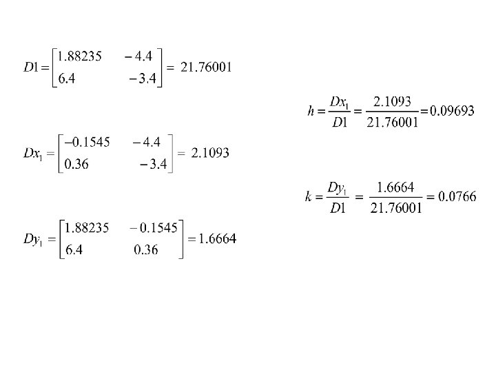
Cramer’s Rule for or the solution of a system of linear equation

• We have from Eqs. 5(a) & 5(b) Or in matrix form

Now let us call And hence we can have (from Cramer’s rule)

• This gives the next approximation, as Using these values we can proceed further for next approximation (better value) This completes the method.

• Solve the given simultaneous equations (up to two iterations)

Q. 2

Solution of Q. 2

• And hence we have the second approximation as • We repeat the process for next approximation

Tridiagonal system of equations (Thomas algorithm)

• In applications, many times we can have system of equations which gives a coefficient matrix of special structure, majority of zeros. Sparse matrices [Upper Triangular & Lower Triangular Matrices] What, If we have a matrix such that except the principal diagonal and its upper and lower diagonal, all the elements are zero…. ? ? ?

Such a matrix is called TRIDIAGONAL MATRIX

Something which looks like…….

Tridiagonal Systems: • The non-zero elements are in the main diagonal, super diagonal and subdiagonal. • aij=0 if |i-j| > 1 CISE 301_Topic 3 25

Mathematically…. • An n×n matrix A is called a tridiagonal matrix if whenever • The system of equations which gives rise to a tridiagonal coefficient matrix is called …. . Tridiagonal System of Equations

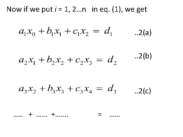
A tridiagonal system for n unknowns may be written as …(1) B. V. P. with second order ODE, Heat conduction equations…. Generate equations like (1)

Which in matrix form can be written as

• Thomas algorithm (named after L. H. Thomas), is a simplified form of Gauss elimination method • Suppose we have a system like And we have to find all the unknowns…

Then Thomas Algo. Gives the values of unknown in the order last to first. . It means first we shall get and then by back substitution, we will get

Where and

Q. 1 Solve the following system of equations

In matrix form CISE 301_Topic 3 34

Section: 2 Finite Difference Interpolation Numerical Integration

Finite Differences Let we have . . (1) which is tabulated for equally spaced values. .

And returns the following values It means

Then we can define the following Differences • Forward Difference DELTA • Backward Difference Nabla • Central Difference delta (lower case)

• Forward Difference First Forward Difference We define the FORWARD DIFFERENCE OPERATOR, denoted by as The expression gives the FIRST FORWARD DIFFERENCE of and the operator is called the FIRST FORWARD DIFFERENCE OPERATOR.

• Notation (First Forward Differences)

Second Forward Differences are given by

• And hence in general the pth Forward Diff. . . (2)

• Forward Difference Table

• Forward Diff. Terms

• Backward differences are defined and denoted by following

Following the concept of Forward Diff. Make a table for Backward Difference up to 5 th Difference

• Central Differences • The central Diff. operator is defined by the following relation Define second third and other central differences And make a central diff. table

• Write the forward Diff. table if…

• Other operators Shift Operator E Average Operator

Shift Operator is the operation of increasing of argument x by h and hence defined by The inverse shift operator is defined by

We have defined the following Differences • Forward Difference DELTA • Backward Difference Nabla • Central Difference delta • Shift Operator E • Average Operator

Relations among the operators

• Proof of (i)

Interpolation Suppose we have following values for y=f(x)

• Interpolation is the technique of estimating the value of a function for any intermediate value of the independent variable • The process of computing the value of the function outside the range is called Extrapolation

Interpolation Equal spaced Unequal Differences Forward Interpolation Newton’s Divided Diff. (Newton’s Fwd. Int. ) Backward Interpolation Lagrange’s Interpolation (Newton’s Bwd. Int. ) Central Diff. Interpolation • Gauss Forward • Gauss Backward • Stirling Formula • Bessel’s Formula • Everett’s Formula

Newton’s Forward Interpolation Suppose the function is tabulated for equally spaced values. . And it takes the following values

• Suppose we have to calculate f(x) at x=x 0+ph (p is any real number), then we have Now we expand the term by Binomial theorem

The above blue colored equation (1) is Newton’s Forward Interpolation Formula Because it contains y 0 and forward differences of y 0

Example Estimate f (3. 17)from the data using Newton Forward Interpolation. x: 3. 1 f(x): 0 3. 2 0. 6 3. 3 1. 0 3. 4 1. 2 61 3. 5 1. 3

Solution 62

Solution 63

Newton’s Backward Interpolation Suppose the function is tabulated for equally spaced values. . And it takes the following values

• Suppose we have to calculate f(x) at x=xn+ph (p is any real number, may be -ve), then we have Now we expand the term by Binomial theorem

NEWTON GREGORY BACKWARD INTERPOLATION FORMULA 66

Example Estimate f(42) from the following data using newton backward interpolation. x: 20 25 30 35 40 45 f(x): 354 332 291 260 231 204 67

Solution Here xn = 45, h = 5, x = 42 and p = - 0. 6 68

Solution 69

Central Difference Formula • Gauss Forward • Gauss Backward • Stirling Formula • Bessel’s Formula • Everett’s Formula

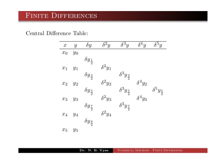
• If y=f(x) is any function, which takes values and returns corresponding values • Then the difference table can be written as

Central Difference table Table-1

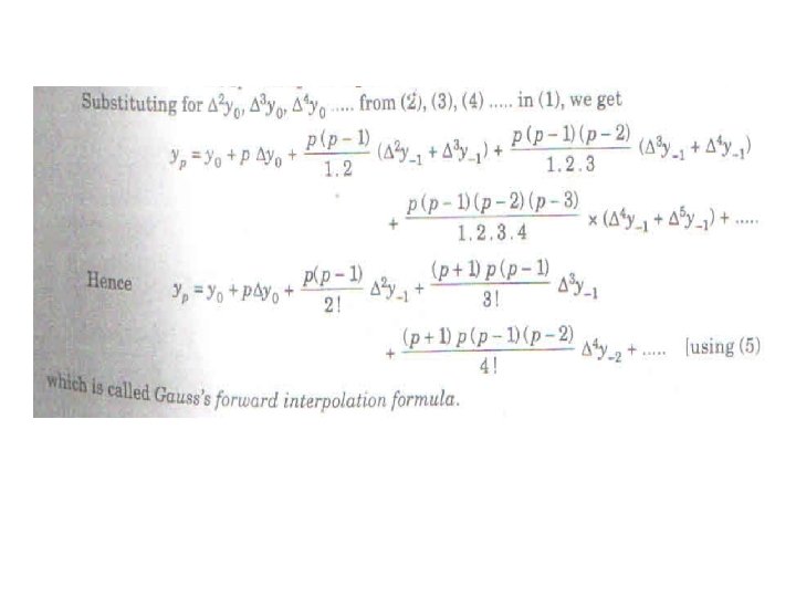
1. GAUSS FORWARD INTERPOLATION FORMULA OR …. . (A) 74

Derivation of Gauss Fwd. Int. Formula We have Newton’s Forward Int. Formula We have following relations (from table)

• Note: (1) Gauss forward formula contains odd differences just below the central line and even differences on the central line (2) Formula is useful to interpolate the value of y for 0<p<1, measured forwardly

Example Find f(30) from the following table values using Gauss forward difference formula: x: 21 25 29 33 37 F(x): 18. 4708 17. 8144 17. 1070 16. 3432 15. 5154 78

Solution f (30) = 16. 9217 79

2. Gauss Backward interpolation formula Again starting with Newton’s Forward Int. Formula

Also we can have And similarly other differences. . Putting these values we finally get this is Gauss Backward Formula

• Note: (1) Gauss Backward formula contains odd differences just above the central line and even differences on the central line • Formula is useful to interpolate the value of y for p lying between -1 & 0

Example Estimate cos 51 42' by Gauss backward interpolation from the following data: x: 50 51 52 53 54 cos x: 0. 6428 0. 6293 0. 6157 0. 6018 0. 5878 83

Solution 84

Solution P(51. 7) = 0. 6198 85

3. STIRLING’S FORMULA • This formula gives the average of the values obtained by Gauss forward and backward interpolation formulae. For using this formula we should have – ½ < p< ½. We can get very good estimates if - ¼ < p < ¼. The formula is: 86

• Stirling Formula (Derivation) [Mean of Gauss Fwd. & Gauss Bkwd] • Eq. (3) is Stirling Formula

• Note: • Stirling Formula contains means of odd differences just above and below the central line and even differences on central line

Example • Using Sterling Formula estimate f (1. 63) from the following table: x: 1. 50 1. 60 1. 70 1. 80 1. 90 f(x): 17. 609 20. 412 23. 045 25. 527 27. 875 Solution X 0 = 1. 60, x = 1. 63, h = 0. 1 89

Solution • Difference table 90

4. BESSELS’ INTERPOLATION FORMULA We have Gauss Fwd. Interpolation Formula as Now we use following relations

• We get the following Bessel’s Formula …. (B)

BESSELS’ INTERPOLATION FORMULA/other way • This formula involves means of even difference on and below the central line and odd difference below the line. • The formula is 93

BESSELS’ INTERPOLATION FORMULA Note • • When p = 1/2 , the terms containing odd differences vanish. Then we get the formula in a more simple form: 94

Example Use Bessels’ Formula to find (46. 24)1/3 from the following table of x 1/3. 95

Solution x 0 = 45, x = 46. 24, h = 4 p = 0. 31 Difference table is: Applying Bessels’ formula, we get (46. 24)1/3 = 3. 5893 96

5. Laplace-Everett’s Formula Gauss’s forward interpolation formula is We eliminate the odd differences in above equation by using the relations

And then to change the terms with negative sign, putting , we obtain …(E) This is known as Laplace-Everett’s formula.

Choice of an interpolation formula The following rules will be found useful: Ø To find a tabulated value near the beginning of the table, use Newton’s forward formula. Ø To find a value near the end of the table, use Newton’s backward formula. Ø To find an interpolated value near the centre of the table, use either Stirling’s or Bessel’s or Everett’s formula.

Choice of central difference Ø If interpolation is required for p lying between and , prefer Stirling’s formula. Ø If interpolation is desired for p lying between and , use Bessel’s or Everett’s formula. Ø Gauss’s Backward interpolation formula is used to interpolate the value of “y” for a negative value of p lying between -1 and 0.

Ø Gauss’s forward interpolation formula is used to interpolate the value of “y” for p (0<p<1) measured forwardly from the origin.

Bessel’s and Everett’s central difference interpolation formula can be obtained by each other by suitable rearrangements.