Numerical Integration SCVASU 1 Numerical Integration Numerical integration

Numerical Integration SCV-ASU 1

Numerical Integration Numerical integration covers several different things, including numerical evaluation of integrals and solutions to ordinary differential equations. In this section, we will talk about numerical evaluation of the definite integrals which will refer to as quadrature. SCV-ASU 2

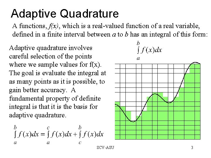
Adaptive Quadrature A functions, f(x), which is a real-valued function of a real variable, defined in a finite interval between a to b has an integral of this form: Adaptive quadrature involves careful selection of the points where we sample values for f(x). The goal is evaluate the integral at as many points as it is possible, to gain better accuracy. A fundamental property of definite integral is that it is the basis for adaptive quadrature. SCV-ASU 3

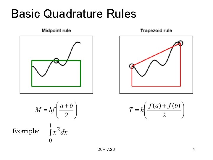
Basic Quadrature Rules Example: SCV-ASU 4

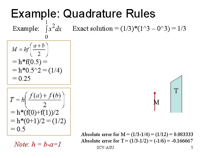
Example: Quadrature Rules Example: Exact solution = (1/3)*(1^3 – 0^3) = 1/3 = h*f(0. 5) = = h*0. 5^2 = (1/4) = 0. 25 T M = h*(f(0)+f(1))/2 = h*(0+1)/2 = (1/2) = 0. 5 Note: h = b-a=1 Absolute error for M = (1/3 -1/4) = (1/12) = 0. 083333 Absolute error for T = (1/3 -1/2) = (-1/6) = -0. 166667 SCV-ASU 5

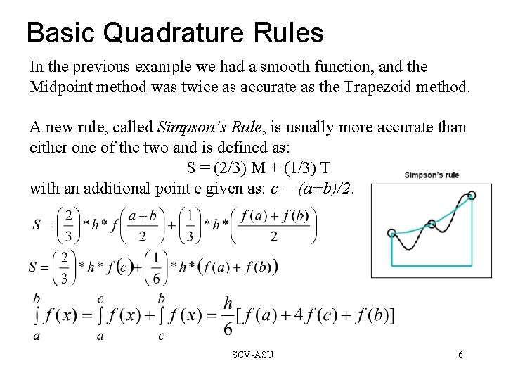
Basic Quadrature Rules In the previous example we had a smooth function, and the Midpoint method was twice as accurate as the Trapezoid method. A new rule, called Simpson’s Rule, is usually more accurate than either one of the two and is defined as: S = (2/3) M + (1/3) T with an additional point c given as: c = (a+b)/2. SCV-ASU 6

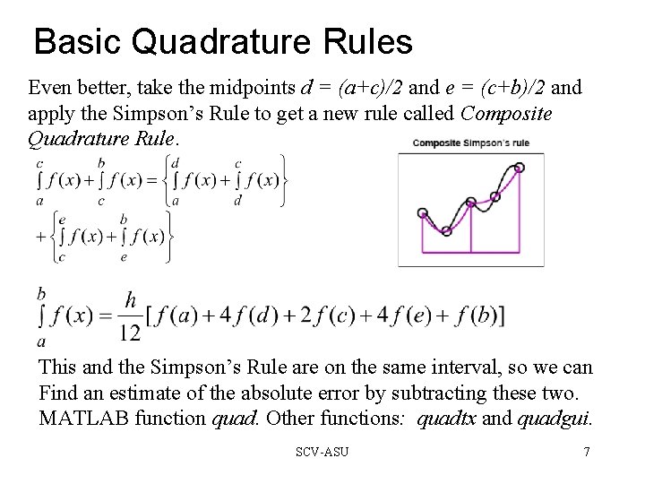
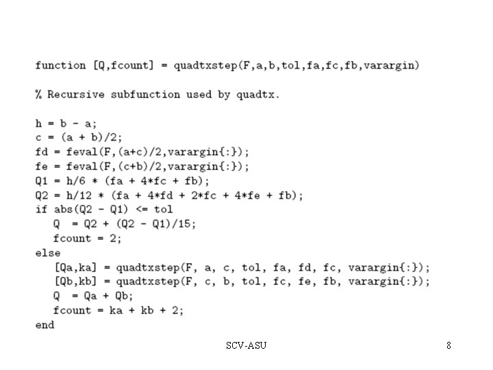
Basic Quadrature Rules Even better, take the midpoints d = (a+c)/2 and e = (c+b)/2 and apply the Simpson’s Rule to get a new rule called Composite Quadrature Rule. This and the Simpson’s Rule are on the same interval, so we can Find an estimate of the absolute error by subtracting these two. MATLAB function quad. Other functions: quadtx and quadgui. SCV-ASU 7

SCV-ASU 8

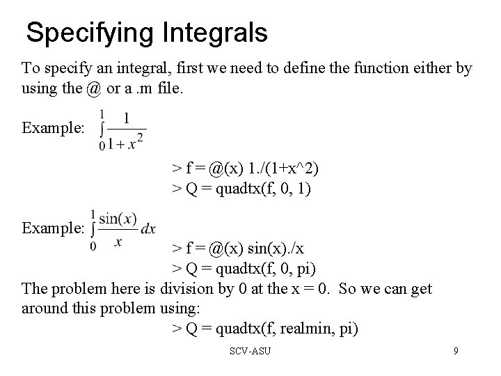
Specifying Integrals To specify an integral, first we need to define the function either by using the @ or a. m file. Example: > f = @(x) 1. /(1+x^2) > Q = quadtx(f, 0, 1) Example: > f = @(x) sin(x). /x > Q = quadtx(f, 0, pi) The problem here is division by 0 at the x = 0. So we can get around this problem using: > Q = quadtx(f, realmin, pi) SCV-ASU 9

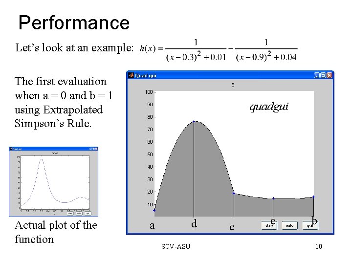
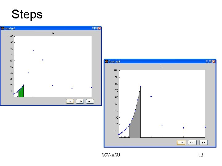
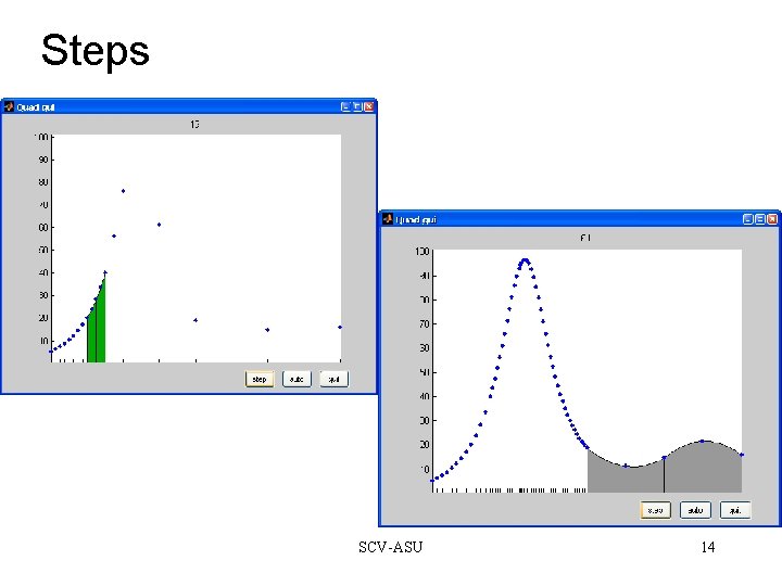
Performance Let’s look at an example: The first evaluation when a = 0 and b = 1 using Extrapolated Simpson’s Rule. Actual plot of the function quadgui d a SCV-ASU c e b 10

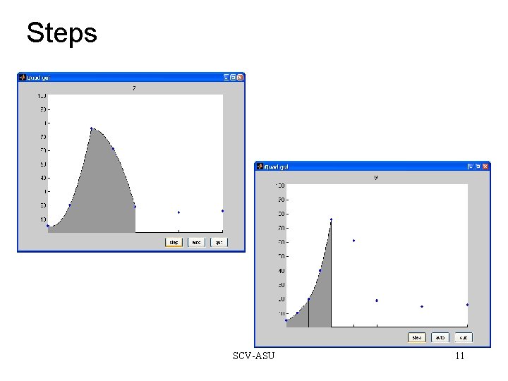
Steps SCV-ASU 11

Steps SCV-ASU 12

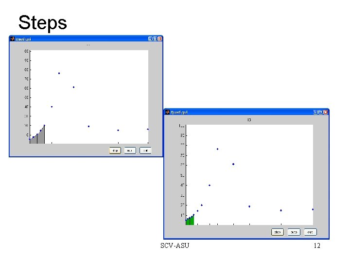
Steps SCV-ASU 13

Steps SCV-ASU 14

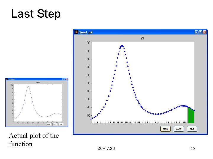
Last Step Actual plot of the function SCV-ASU 15

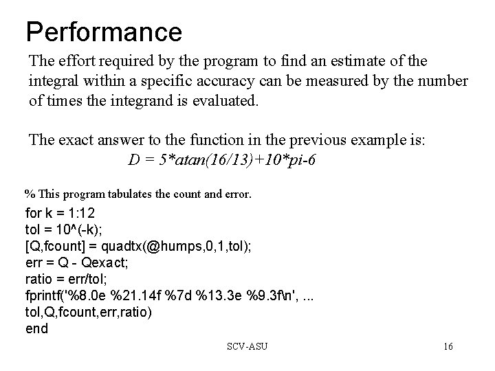
Performance The effort required by the program to find an estimate of the integral within a specific accuracy can be measured by the number of times the integrand is evaluated. The exact answer to the function in the previous example is: D = 5*atan(16/13)+10*pi-6 % This program tabulates the count and error. for k = 1: 12 tol = 10^(-k); [Q, fcount] = quadtx(@humps, 0, 1, tol); err = Q - Qexact; ratio = err/tol; fprintf('%8. 0 e %21. 14 f %7 d %13. 3 e %9. 3 fn', . . . tol, Q, fcount, err, ratio) end SCV-ASU 16

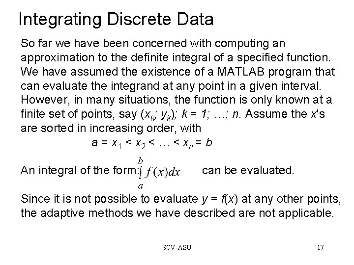
Integrating Discrete Data So far we have been concerned with computing an approximation to the definite integral of a specified function. We have assumed the existence of a MATLAB program that can evaluate the integrand at any point in a given interval. However, in many situations, the function is only known at a finite set of points, say (xk; yk); k = 1; …; n. Assume the x's are sorted in increasing order, with a = x 1 < x 2 < … < xn = b An integral of the form: can be evaluated. Since it is not possible to evaluate y = f(x) at any other points, the adaptive methods we have described are not applicable. SCV-ASU 17

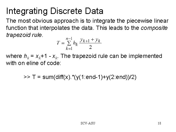
Integrating Discrete Data The most obvious approach is to integrate the piecewise linear function that interpolates the data. This leads to the composite trapezoid rule. where hk = xk+1 - xk. The trapezoid rule can be implemented with on eline of code: >> T = sum(diff(x). *(y(1: end-1)+y(2: end))/2) SCV-ASU 18