H E Hamiltonian for the H atom H

Hψ = E ψ Hamiltonian for the H atom

Hψ = E ψ H = H 1 + H 2 Separated H atoms

H = H 1 + H 2 + H 12 extra term due to interaction as the atoms get close

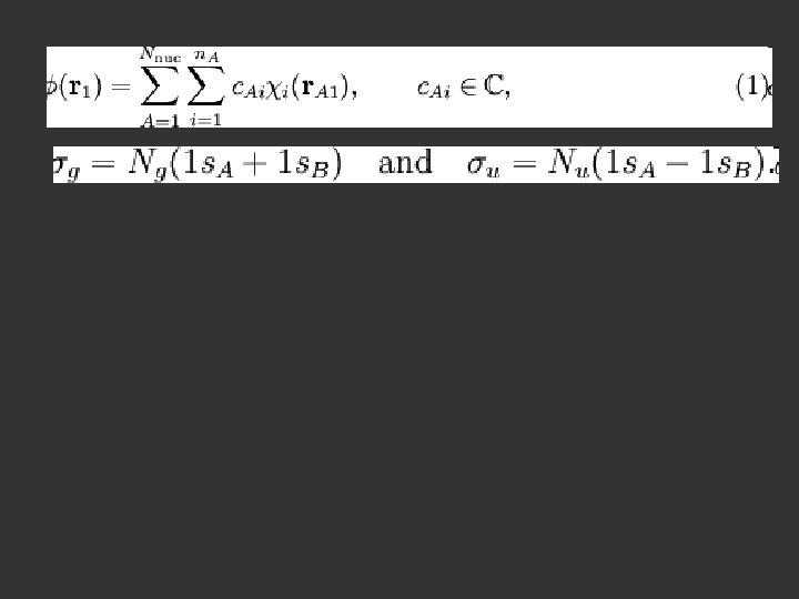
LCAO-MO Approximation Linear Combination of Atomic Orbitals – Molecular Orbital Approximation

LCAO-MO Approximation Ψ = Σ i c i φi

LCAO-MO Approximation Ψ = Σ i c i φi Ψ molecular wavefunction

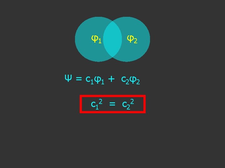
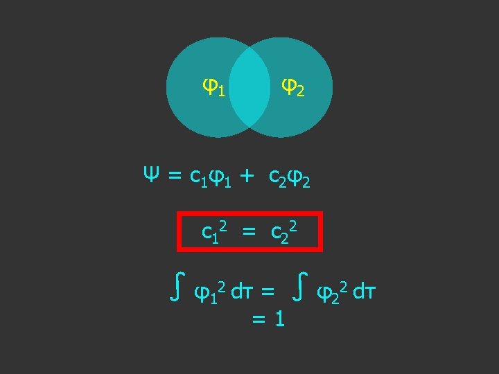
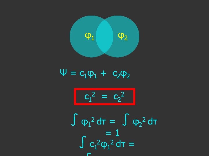
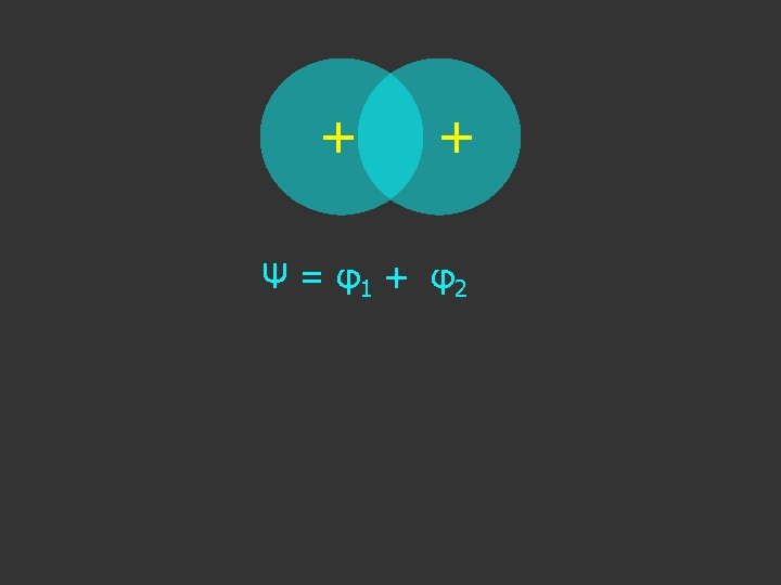
In this simple case: Ψ = c 1 φ1 + c 2 φ2

LCAO-MO Approximation Ψ = Σ i c i φi Ψ Σi molecular wavefunction summation operator

LCAO-MO Approximation Ψ = Σ i c i φi Ψ molecular wavefunction Σi summation operator ci orbital coefficient

LCAO-MO Approximation Ψ = Σ i c i φi Ψ molecular wavefunction Σi summation operator ci orbital coefficient φi atomic orbital

1 a T+V→H

1 a T+V→H V = -1/ra 1

a Distance apart ra 1 Coulomb potential V = -eae 1/ra 1 V = -1/ra 1 1

1 a T+V→H V = -1/ra 1 Setting charge e 2 = 1

1 a T+V→H V = -1/ra 1 Setting charge e 2 = 1 Coulombic Potential

1 NOTE The negative sign as energy lowered a T+V→H V = - 1/ra 1 Setting charge e 2 = 1 Coulombic Potential

1 2 a b T+V→H V = -1/ra 1 - 1/rb 2

1 a 2 b V = -1/ra 1 - 1/rb 2

1 a 2 b V = -1/ra 1 - 1/rb 2 + 1/rab

1 a 2 b V = -1/ra 1 - 1/rb 2 + 1/rab + 1/r 12

1 2 a b V = -1/ra 1 - 1/rb 2 + 1/rab + 1/r 12 - 1/ra 2

1 a 2 b V = -1/ra 1 - 1/rb 2 + 1/rab + 1/r 12 - 1/ra 2 - 1/rb 1

H = H 1 + H 2 + H 12 Hψ = E ψ Ψ = c 1 φ1 + c 2 φ2 LCAO MO Approximation Linear Combination of Atomic Orbitals

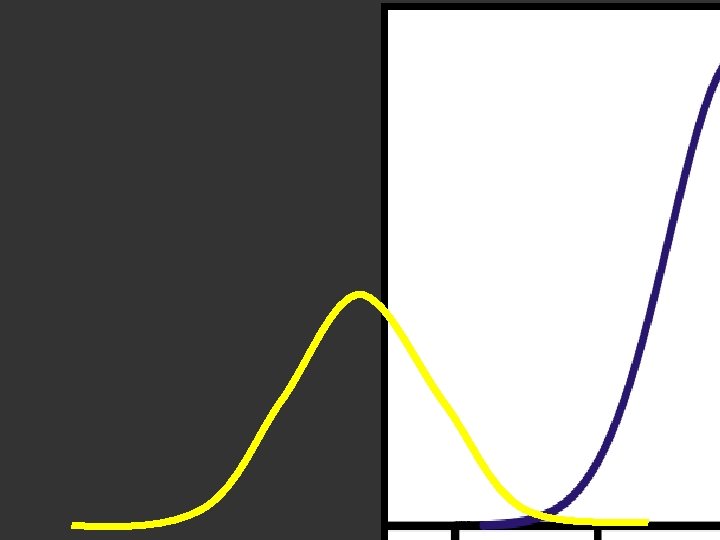
Electron Density is given by Ψ 2 or Ψ*Ψ

c 1 2 = c 2 2

c 1 2 = c 2 2 c 1 = ±? c 2

c 1 2 = c 2 2 c 1 = ±c 2

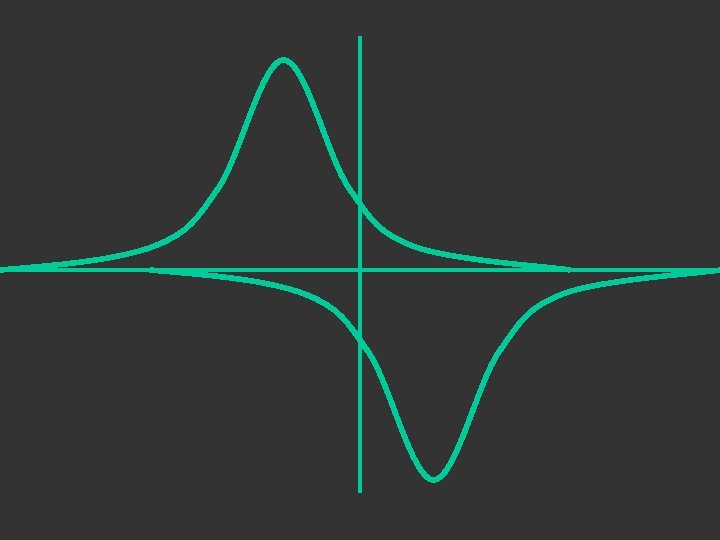
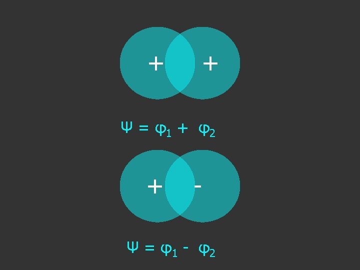
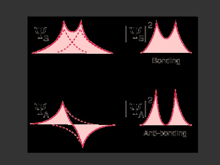
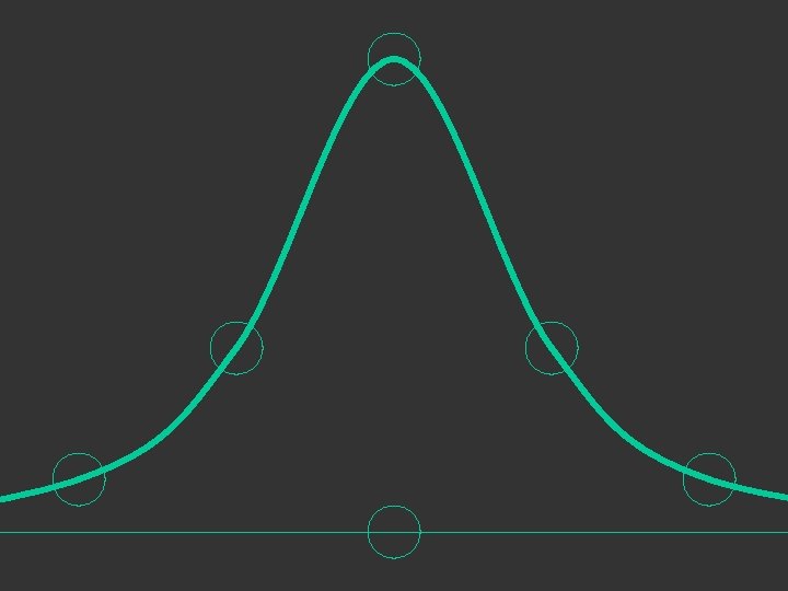
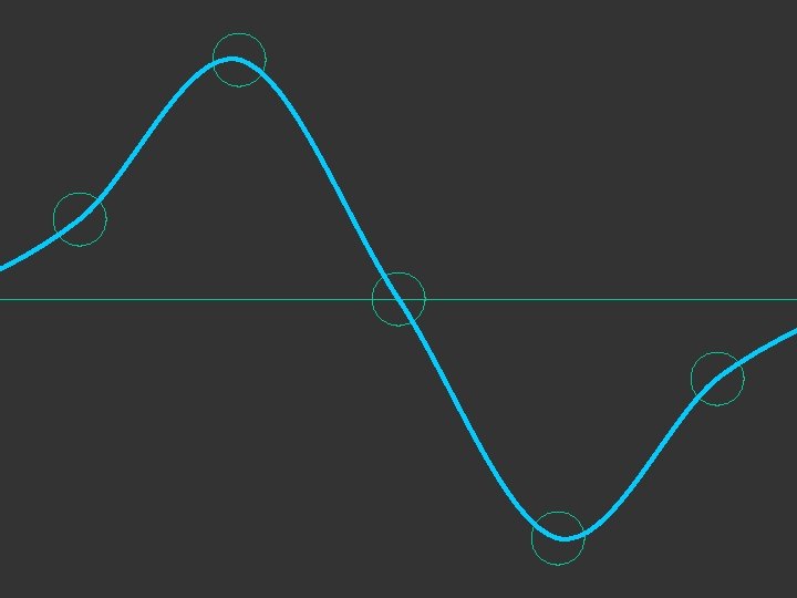
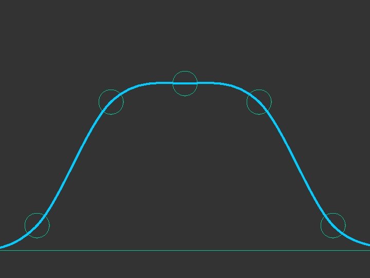
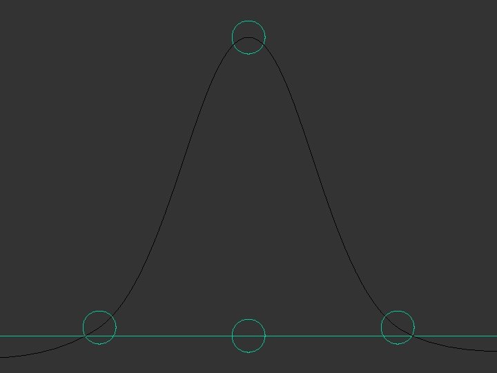
Electron Wavefunction Ψ

Electron Wavefunction Ψ

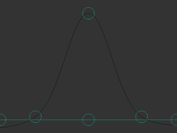
Bonding Orbital Electron Density Ψ 2

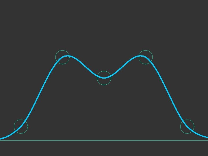
Antibonding Orbital Electron Density Ψ 2

H = H 1 + H 2 + H 12

H = H 1 + H 2 + H 12

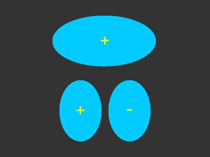
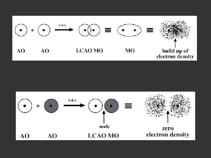
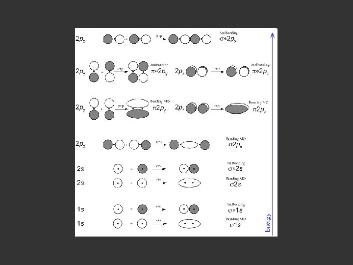
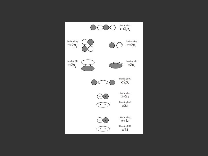
1 sa + 1 sb + σbonding σ + - 1 sa - 1 sb σantibonding σ*

+ + - The + and – signs are not charge signs they are phase indicators

+ - + Protons pulled towards each other by the buildup of –ve charge in the centre

+ + - + + Protons pulled towards each other by the buildup of –ve charge in the centre Protons repelled as little negative charge build up in the centre

+ + - + + Protons pulled towards each other by the buildup of –ve charge in the centre Protons repelled as little negative charge build up in the centre Note - Now we are discussing the charges

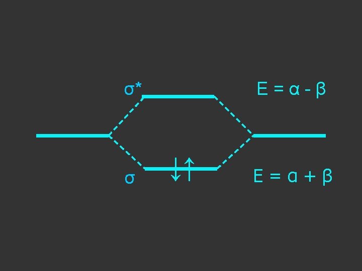
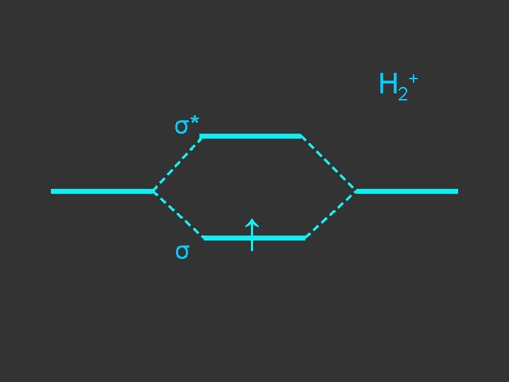
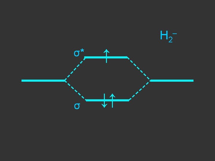
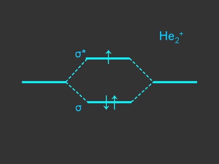
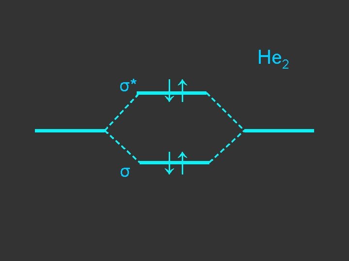
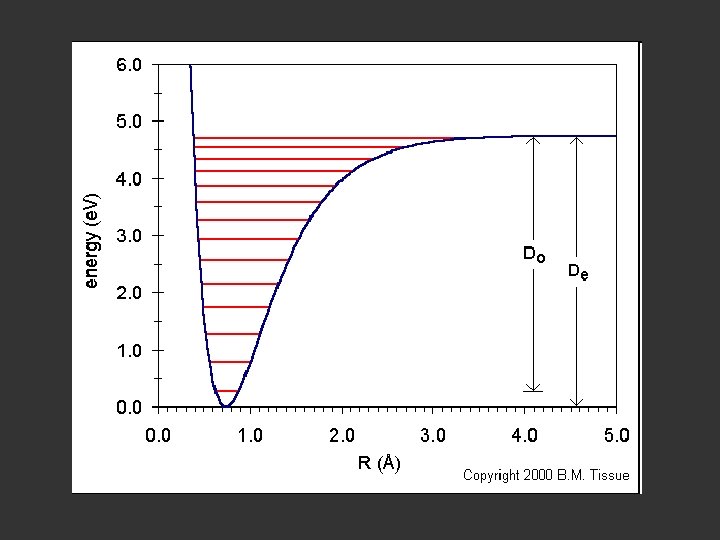
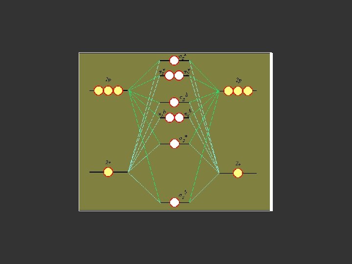
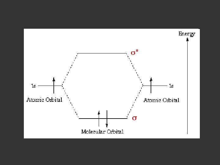
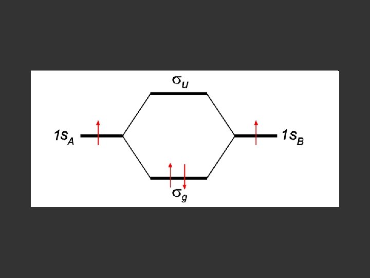
Separate atoms ↑ ↑

At the bond separation the bonding and antibonding orbitals split apart in energy ↑ ↑

The electrons pair up in the lower level – energy is gained - relative to the separate atoms and a stable molecule is formed σ* ↑ ↑ σ ↓↑

E = α - β ↓↑ E=α+β Note β the stabilisation energy is –ve

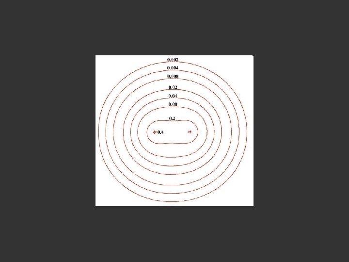
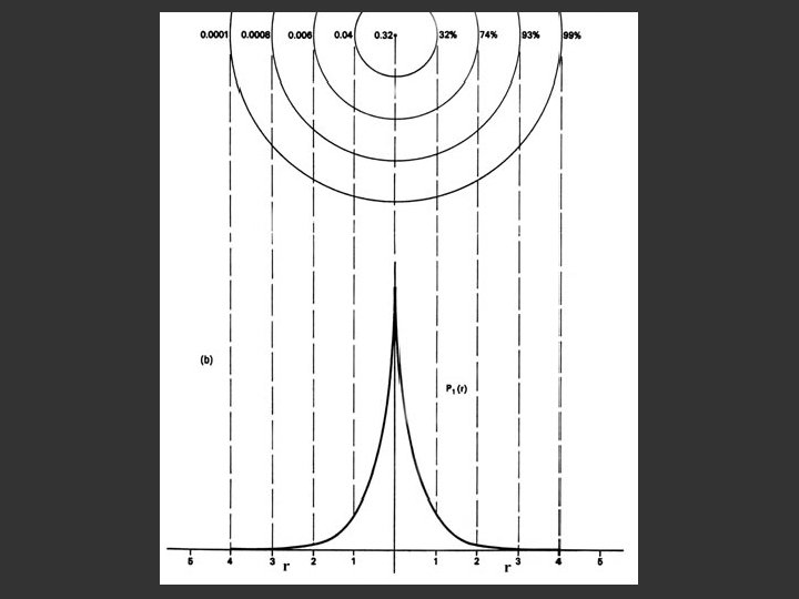
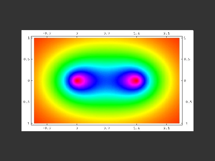
A contour map of the electron density distribution (or the molecular charge distribution) for H 2 in a plane containing the nuclei.

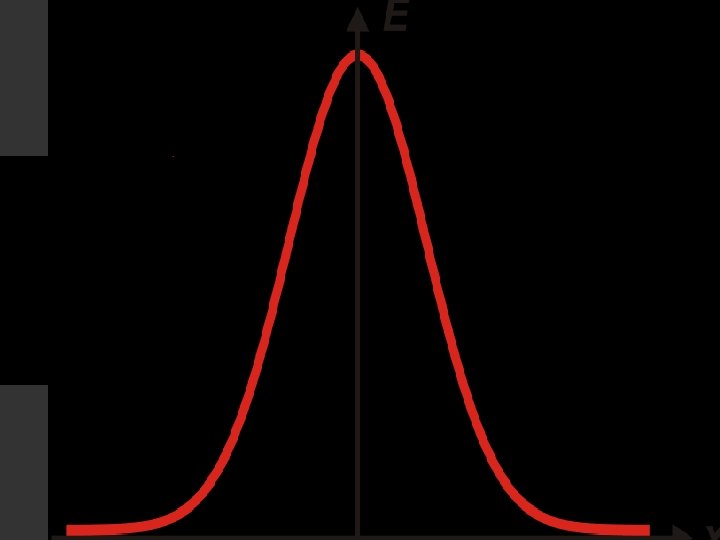
Fig. 6 -2. A contour map of the electron density distribution (or the molecular charge distribution) for H 2 in a plane containing the nuclei. Also shown is a profile of the density distribution along the internuclear axis. The internuclear separation is 1. 4 au. The values of the contours increase in magnitude from the outermost one inwards towards the nuclei. The values of the contours in this and all succeeding diagrams are given in au; 1 au = e/ao 3 = 6. 749 e/Å3.

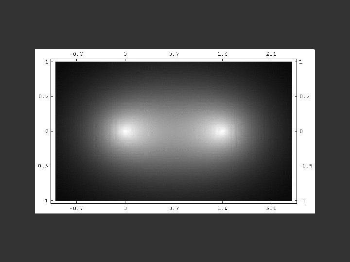
Hydrogen. The two electrons in the hydrogen molecule may both be accommodated in the 1 sg orbital if their spins are paired and the molecular orbital configuration for H 2 is 1 sg 2. Since the 1 sg orbital is the only occupied orbital in the ground state of H 2, the density distribution shown previously in Fig. 62 for H 2 is also the density distribution for the 1 sg orbital when occupied by two electrons. The remarks made previously regarding the binding of the nuclei in H 2 by the molecular charge distribution apply directly to the properties of the 1 sg charge density. Because it concentrates charge in the binding region and exerts an attractive force on the nuclei the 1 sg orbital is classified as a bonding orbital. http: //www. chemistry. mcmaster. ca/esam/Chapter_3/section_2. html

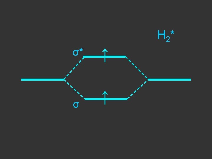
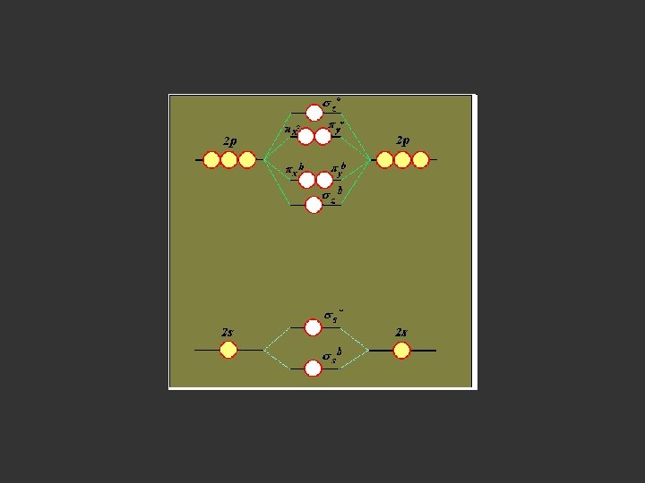
Hydrogen. II Excited electronic configurations for molecules may be described and predicted with the same ease within the framework of molecular orbital theory as are the excited configurations of atoms in the corresponding atomic orbital theory. For example, an electron in H 2 may be excited to any of the vacant orbitals of higher energy indicated in the energy level diagram. The excited molecule may return to its ground configuration with the emission of a photon. The energy of the photon will be given approximately by the difference in the energies of the excited orbital and the 1 sg ground state orbital. Thus molecules as well as atoms will exhibit a line spectrum. The electronic line spectrum obtained from a molecule is, however, complicated by the appearance of many accompanying side bands. These have their origin in changes in the vibrational energy of the molecule which accompany the change in electronic energy.

Electron Density Ψ*Ψ

http: //tannerm. com/diatomic. htm

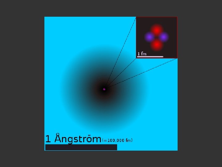
The nucleus is the very dense region consisting of nucleons (protons and neutrons) at the center of an atom. Almost all of the mass in an atom is made up from the protons and neutrons in the nucleus, with a very small contribution from the orbiting electrons. The diameter of the nucleus is in the range of 1. 6 fm (1. 6 × 10− 15 m) (for a proton in light hydrogen) to about 15 fm (for the heaviest atoms, such as uranium). These dimensions are much smaller than the diameter of the atom itself, by a factor of about 23, 000 (uranium) to about 145, 000 (hydrogen). The branch of physics concerned with studying and understanding the atomic nucleus, including its composition and the forces which bind it together, is called nuclear physics.

1 2 a b T+V→H V = -1/ra 1 - 1/rb 2 H 12 = 1/rab + 1/r 12 - 1/ra 2 + 1/rb 1 Setting charge e 2 = 1

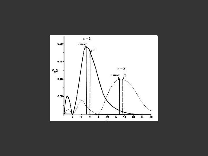
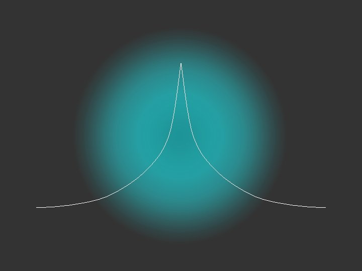
The wave function is usually represented by ψ

2 The electron density is given by ψ

probability = ψ2 Electron Density Radius r

- jpg - classweb. gmu. edu/. . . /graphics/H 2 -orbitals. jpg Image may be subject to copyright.