Advanced Numerical Methods S A Sahu Code AMC

Advanced Numerical Methods (S. A. Sahu) Code: AMC 51151

Syllabus We can divide our syllabus in following four major sections: 1. Method of solution of system of equations Solution of Non-linear Simultaneous Equations (Newton-Raphson Method) Tridiagonal system of equations (Thomas algorithm)

2. Numerical Integration Evaluation of Double & Triple Integrals (a) Constant Limit Simpson’s Rule (b) Variable Limit & Trapezoidal Rule

3. Methods of Interpolation Ø Newton’s F/W and B/W formula Ø Gauss’s F/W and B/W formula Ø Bessel’s Formula Ø Stirling Formula Ø Lagrange’s Interpolation Formula Ø Newton’s Divided Difference Formula

4. Numerical Solution of Differential Equations O. D. E. • First Order & Higher Ordinary Diffe. Eqs. • Initial Value & Boundary Value Problems P. D. E. • Laplace & Poisson Equations • Heat Conduction • Wave Equations

Solution of Non-linear Simultaneous Equations (Newton-Raphson Method)

This Method is extension of N-R Method for Non-Linear Equation • Method for Simultaneous equations: Suppose we are given the following Simultaneous equations …(1) Why simultaneous. . ?

We consider that And be the first approximation be the real roots It means, we must have : …. (2)

Now we expand the relation, we had in eq. (2) Using Taylor Series Expansion (3) (similarly for ) Now since h and k are very small, we can neglect the terms containing (or )and higher order terms…

• Now, eq. (2), eq. (3) and assumption suggests . . (4 a) . . (4 b)

• Or simply: … 5(a) . . 5(b) Let us say

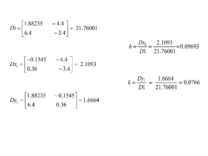
Cramer’s Rule for or the solution of a system of linear equation

• We have from Eqs. 5(a) & 5(b) Or in matrix form

Now let us call And hence we can have (from Cramer’s rule)

• This gives the next approximation, as Using these values we can proceed further for next approximation (better value) This completes the method.

• Solve the given simultaneous equations (up to two iterations)

Q. 2

Solution of Q. 2

• And hence we have the second approximation as • We repeat the process for next approximation

Tridiagonal system of equations (Thomas algorithm)

• In applications, many times we can have system of equations which gives a coefficient matrix of special structure, majority of zeros. Sparse matrices [Upper Triangular & Lower Triangular Matrices] What, If we have a matrix such that except the principal diagonal and its upper and lower diagonal, all the elements are zero…. ? ? ?

Such a matrix is called TRIDIAGONAL MATRIX

Something which looks like…….

Tridiagonal Systems: • The non-zero elements are in the main diagonal, super diagonal and subdiagonal. • aij=0 if |i-j| > 1 CISE 301_Topic 3 25

Mathematically…. • An n×n matrix A is called a tridiagonal matrix if whenever • The system of equations which gives rise to a tridiagonal coefficient matrix is called …. . Tridiagonal System of Equations

A tridiagonal system for n unknowns may be written as …(1) B. V. P. with second order ODE, Heat conduction equations…. Generate equations like (1)

Which in matrix form can be written as

• Thomas algorithm (named after L. H. Thomas), is a simplified form of Gauss elimination method • Suppose we have a system like And we have to find all the unknowns…

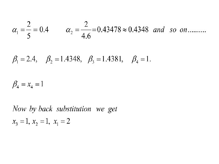
Then Thomas Algo. Gives the values of unknown in the order last to first. . It means first we shall get substitution, we will get and then by back

Where and

Q. 1 Solve the following system of equations

In matrix form CISE 301_Topic 3 34

Section: 2 Finite Difference Interpolation Numerical Integration

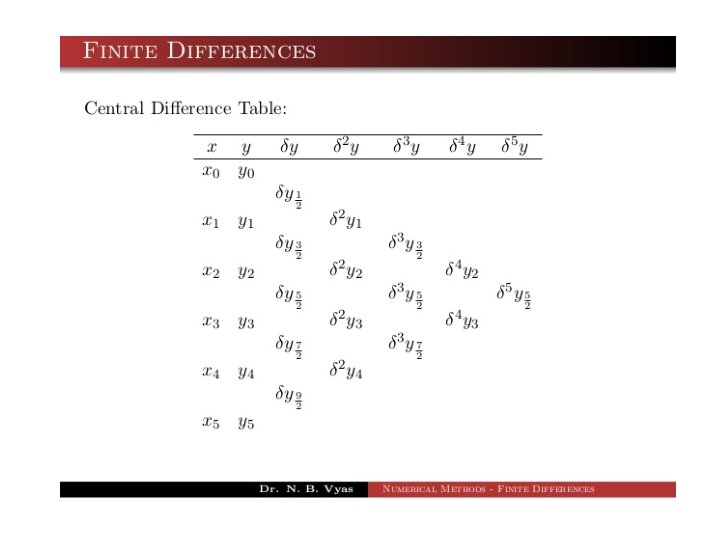
Finite Differences Let we have. . (1) which is tabulated for equally spaced values. .

And returns the following values It means

Then we can define the following Differences • Forward Difference DELTA • Backward Difference Nabla • Central Difference delta (lower case)

• Forward Difference First Forward Difference We define the FORWARD DIFFERENCE OPERATOR, denoted by as The expression gives the FIRST FORWARD DIFFERENCE of and the operator is called the FIRST FORWARD DIFFERENCE OPERATOR.

• Notation (First Forward Differences)

Second Forward Differences are given by

• And hence in general the pth Forward Diff. . . (2)

• Forward Difference Table

• Forward Diff. Terms

• Backward differences are defined and denoted by following

Following the concept of Forward Diff. Make a table for Backward Difference up to 5 th Difference

• Central Differences • The central Diff. operator following relation is defined by the Define second third and other central differences And make a central diff. table

• Write the forward Diff. table if…

• Other operators Shift Operator E Average Operator

Shift Operator is the operation of increasing of argument x by h and hence defined by The inverse shift operator is defined by

We have defined the following Differences • Forward Difference DELTA • Backward Difference Nabla • Central Difference delta • Shift Operator • Average Operator E

Relations among the operators

• Proof of (i)

Interpolation Suppose we have following values for y=f(x)

• Interpolation is the technique of estimating the value of a function for any intermediate value of the independent variable • The process of computing the value of the function outside the range is called Extrapolation

Interpolation Equal spaced Unequal Differences Forward Interpolation Newton’s Divided Diff. (Newton’s Fwd. Int. ) Backward Interpolation Lagrange’s Interpolation (Newton’s Bwd. Int. ) Central Diff. Interpolation • Gauss Forward • Gauss Backward • Stirling Formula • Bessel’s Formula • Everett’s Formula

Newton’s Forward Interpolation Suppose the function is tabulated for equally spaced values. . And it takes the following values

• Suppose we have to calculate f(x) at x=x 0+ph (p is any real number), then we have Now we expand the term by Binomial theorem

The above blue colored equation (1) is Newton’s Forward Interpolation Formula Because it contains y 0 and forward differences of y 0

Example Estimate f (3. 17)from the data using Newton Forward Interpolation. x: 3. 1 f(x): 0 3. 2 0. 6 3. 3 1. 0 3. 4 1. 2 61 3. 5 1. 3

Solution 62

Solution 63

Newton’s Backward Interpolation Suppose the function is tabulated for equally spaced values. . And it takes the following values

• Suppose we have to calculate f(x) at x=xn+ph (p is any real number, may be -ve), then we have Now we expand the term by Binomial theorem

NEWTON GREGORY BACKWARD INTERPOLATION FORMULA 66

Example Estimate f(42) from the following data using newton backward interpolation. x: 20 25 30 35 40 45 f(x): 354 332 291 260 231 204 67

Solution Here xn = 45, h = 5, x = 42 and p = - 0. 6 68

Solution 69

Central Difference Formula • Gauss Forward • Gauss Backward • Stirling Formula • Bessel’s Formula • Everett’s Formula

• If y=f(x) is any function, which takes values and returns corresponding values • Then the difference table can be written as

Central Difference table Table-1

1. GAUSS FORWARD INTERPOLATION FORMULA OR …. . (A) 74

Derivation of Gauss Fwd. Int. Formula We have Newton’s Forward Int. Formula We have following relations (from table)

• Note: (1) Gauss forward formula contains odd differences just below the central line and even differences on the central line (2) Formula is useful to interpolate the value of y for 0<p<1, measured forwardly

Example Find f(30) from the following table values using Gauss forward difference formula: x: 21 25 29 33 37 F(x): 18. 4708 17. 8144 17. 1070 16. 3432 15. 5154 78

Solution f (30) = 16. 9217 79

2. Gauss Backward interpolation formula Again starting with Newton’s Forward Int. Formula

Also we can have And similarly other differences. . Putting these values we finally get this is Gauss Backward Formula

• Note: (1) Gauss Backward formula contains odd differences just above the central line and even differences on the central line • Formula is useful to interpolate the value of y for p lying between -1 & 0

Example Estimate cos 51 42' by Gauss backward interpolation from the following data: x: cos x: 50 0. 6428 51 52 53 54 0. 6293 0. 6157 0. 6018 0. 5878 83

Solution 84

Solution P(51. 7) = 0. 6198 85

3. STIRLING’S FORMULA • This formula gives the average of the values obtained by Gauss forward and backward interpolation formulae. For using this formula we should have – ½ < p< ½. We can get very good estimates if - ¼ < p < ¼. The formula is: 86

• Stirling Formula (Derivation) [Mean of Gauss Fwd. & Gauss Bkwd] • Eq. (3) is Stirling Formula

• Note: • Stirling Formula contains means of odd differences just above and below the central line and even differences on central line

Example • Using Sterling Formula estimate f (1. 63) from the following table: x: 1. 50 1. 60 1. 70 1. 80 1. 90 f(x): 17. 609 20. 412 23. 045 25. 527 27. 875 Solution X 0 = 1. 60, x = 1. 63, h = 0. 1 89

Solution • Difference table 90

4. BESSELS’ INTERPOLATION FORMULA We have Gauss Fwd. Interpolation Formula as Now we use following relations

• We get the following Bessel’s Formula …. (B)

BESSELS’ INTERPOLATION FORMULA/other way • This formula involves means of even difference on and below the central line and odd difference below the line. • The formula is 93

BESSELS’ INTERPOLATION FORMULA Note • • When p = 1/2 , the terms containing odd differences vanish. Then we get the formula in a more simple form: 94

Example Use Bessels’ Formula to find (46. 24)1/3 from the following table of x 1/3. 95

Solution x 0 = 45, x = 46. 24, Difference table is: h = 4 p = 0. 31 Applying Bessels’ formula, we get (46. 24)1/3 = 3. 5893 96

5. Laplace-Everett’s Formula Gauss’s forward interpolation formula is We eliminate the odd differences in above equation by using the relations

And then to change the terms with negative sign, putting , we obtain …(E) This is known as Laplace-Everett’s formula.

Choice of an interpolation formula The following rules will be found useful: Ø To find a tabulated value near the beginning of the table, use Newton’s forward formula. Ø To find a value near the end of the table, use Newton’s backward formula. Ø To find an interpolated value near the centre of the table, use either Stirling’s or Bessel’s or Everett’s formula.

Choice of central difference Ø If interpolation is required for p lying between and , prefer Stirling’s formula. Ø If interpolation is desired for p lying between and , use Bessel’s or Everett’s formula. Ø Gauss’s Backward interpolation formula is used to interpolate the value of “y” for a negative value of p lying between -1 and 0.

Ø Gauss’s forward interpolation formula is used to interpolate the value of “y” for p (0<p<1) measured forwardly from the origin.

Bessel’s and Everett’s central difference interpolation formula can be obtained by each other by suitable rearrangements.

Interpolation for irregular (un equal) interval

Interpolation produces a function that matches the given data exactly. The function then can be utilized to approximate the data values at intermediate points.

WHAT IS INTERPOLATION? Given (x 0, y 0), (x 1, y 1), …, (xn, yn), finding the value of ‘y’ at a value of ‘x’ in (x 0, xn) is called interpolation. 105

An Interpolating Function for a set of data: {(x 1, y 1), (x 2, y 2), (x 3, y 3)…(xm, ym)} is a function f(x) that satisfies: f(x 1) = y 1 f(x 2) = y 2 f(x 3) = y 3. . . f(xm) = ym

Steps in Interpolation Ø Given data points Ø Obtain a function, P(x) Ø P(x) goes through the data points Ø Use P(x) Ø To estimate values at intermediate points

Interpolating Data with a Function The problem we will be discussing is how if you are given a set of data points {(x 1, y 1), (x 2, y 2), (x 3, y 3)…(xm, ym)} , can an interpolating function f(x) be constructed to fit the data. Polynomial Interpolation A Polynomial Interpolation for a set of data is an interpolating function f(x) such that f(x) is a polynomial. f(x) = anxn + an-1 xn-1 + an-2 xn-2 + … + a 1 x + a 0 Degree of Polynomial Interpolation The degree of a polynomial p(x) = anxn + an-1 xn-1 + an-2 xn-2 + … + a 1 x + a 0 is the largest exponent with a non-zero coefficient. For the given p(x) its degree is n.

In previous equation : No. of terms in polynomial Degree of Polynomial n+1 n The degree of the polynomial required is less than the number of data points. In general a data set of m points will require a polynomial of degree m-1 or less.

LAGRANGE'S INTERPOLATION FORMULA This is Nth degree polynomial approximation formula to the function f(x), which is known at some discrete points xi, (i = 0, 1, 2. . n)

Idea of Lagrange interpolation by an Example

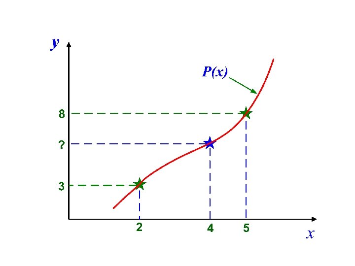
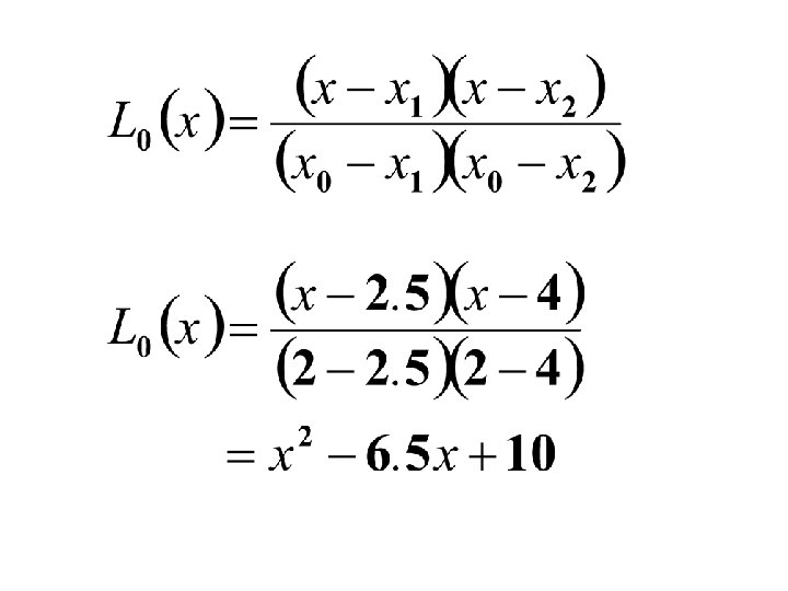
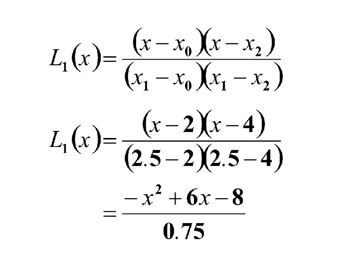
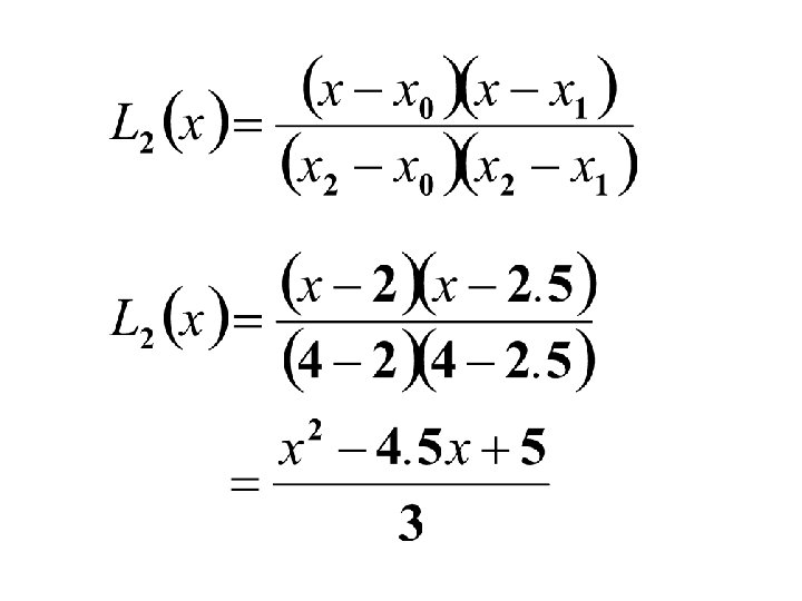
Given data points: At x 0 = 2, y 0 = 3 and at x 1 = 5, y 1 = 8 Find the following: At x = 4, y = ?

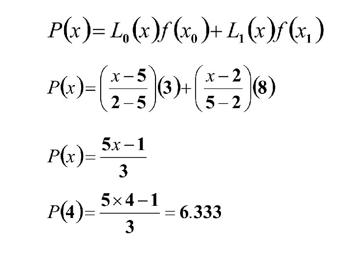
P(x) should satisfy the following conditions: P(x = 2) = 3 and P(x = 5) = 8 (y 0 and y 1) P(x) can satisfy the above conditions if at x = x 0 = 2, L 0(x) = 1 and L 1(x) = 0 and at x = x 1= 5, L 0(x) = 0 and L 1(x) = 1

At x = x 0 = 2, L 0(x) = 1 and L 1(x) = 0 and at x = x 1= 5, L 0(x) = 0 and L 1(x) = 1 The conditions can be satisfied if L 0(x) and L 1(x) are defined in the following way.

Lagrange Interpolating Polynomial

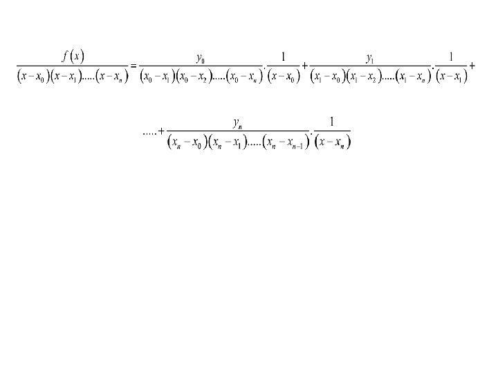
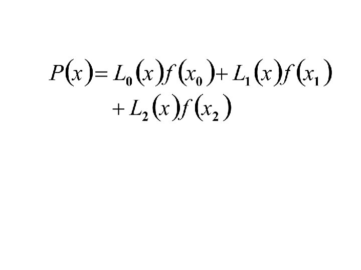
LAGRANGIAN FORMULA Lagrangian interpolating polynomial is given by n f n ( x ) = å Li ( x ) f ( xi ) i =0 where ‘ n ’ in f n (x ) stands for the n th order polynomial that approximates the function y = f (x ) given at (n + 1) data points as (x 0 , y 0), (x 1 , y 1), . . . , (x n -1 , y n -1) , (x n , y n) , and n Li ( x ) = Õ j =0 j ¹i x - xj xi - x j (i = 0, 1, 2. . n) Li (x ) is a weighting function that includes a product of (n - 1) terms with terms of j = i omitted. 119

Lagrange Interpolating Polynomials by Lale Yurttas, Texas A&M University Chapter 18 120

The Lagrange interpolating polynomial is simply a reformulation of the Newton’s polynomial that avoids the computation of divided differences

Lagrange Interpolating Polynomial The Lagrange Form of an interpolating polynomial makes use of elimination of terms and cancellation to fit the data set. Data Set Polynomial

Proof: (Lagrange Interpolation Formula) Let be a function which takes the values Since there are n+1 pairs of values of x and y, we can represent f(x) by a polynomial in x of degree n. let this polynomials of the form ……. (2) Putting Similarly putting in (2), we get in (2), we have

Proceeding in the same way. We find Subtituting the value in (2), we get …. (A) This is known as Lagrange’s interpolation formula for unequal intervals.

observations Ø Lagrange’s formula can be applied whether the values are equally spaced or not. It is easy to remember but quite cumbersome to apply. Ø This formula can also be used to split the given function into partial fractions. for on dividing both sides of (1) by we get

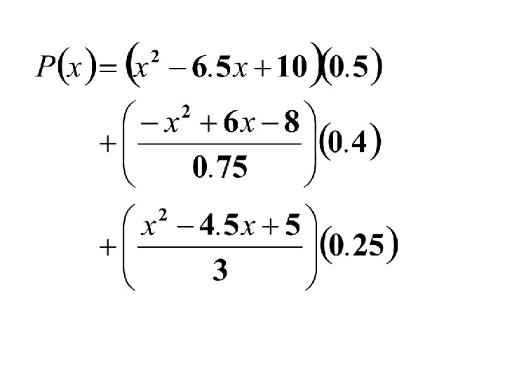
Find the Lagrange Interpolating Polynomial using the three given points. And hence find f(3) Y=? If x=3

The three given points were taken from the function

An approximation can be obtained from the Lagrange Interpolating Polynomial as

• Example : Given the values 5 7 11 13 17 150 392 1452 2366 5202 Evaluate f(9), using Lagrange’s formula Solution: Here

Putting and substituting the values in Lagrange’s formula, we get

Example A manufacturer of thermistors* makes the following observations on a thermistor. Determine the temperature corresponding to 754. 8 ohms using the Lagrangian method for interpolation. R T Ohm C 1101. 0 25. 113 911. 3 30. 131 636. 0 40. 120 451. 1 50. 128 A thermistor is a type of resistor whose resistance is dependent on temperature Thermistor= thermal + resistor 137

Solution 138

Solution 139

Solution 140

Exercise : Use Lagrange’s formula to find the form of f(x), given 0 2 3 6 648 704 729 792 Exercise: Use Lagrange’s formula to find the of y when x=10, if the following values of x and y are given: 5 6 9 11 12 13 14 16

Introduction to Divided Differences A new algebraic representation for Ø Suppose that is the nth Lagrange polynomial that agrees with the function f at the distinct numbers. Ø Although this polynomial is unique, there alternate algebraic representations that are useful in certain situations.

Now if we try to use the divided differences of f with respect to to express in the form for appropriate constants

• To determine the first of these constants, , note that if is written in the form of the above equation, then evaluating at leaves only the constant term ; that is,

Similarly, when is evaluated at , the only nonzero terms in the evaluation of are the constant and linear terms,

• We now introduce the divided-difference notation, • The zero divided difference of the function f with respect to , denoted , is simply the value of f at : • The remaining divided differences are defined by the formula

The first divided difference of f with respect to and is denoted and defined as The second divided difference, defined as , is

Ø Similarly, after the (k − 1)st divided differences, and have been determined, the kth divided difference relative to is Ø The process ends with the single nth divided difference,

Generating the Divided Difference Table

Newton’s Divided Difference Formula Let be the values of corresponding to the arguments. Then from the definition of divided difference, we have So that …. . (1) Again which gives

Substituting the values of in (1), we get ……(2) Proceeding in this manner, we get …(3) Which is called the Newton’s general interpolation formula with divided differences.

• Example : Given the values 5 7 11 13 17 150 392 1452 2366 5202 Evaluate f(9), using Newton’s Divided Difference Formula

Previous exercise solution: By using Newton’s divided difference formula. x y 5 150 7 392 11 1452 13 2366 17 5202 1 st divided difference 121 265 457 709 2 nd divided difference 24 32 42 3 rd divided difference 1 1

Taking in the Newton’s divided difference formula, we obtain

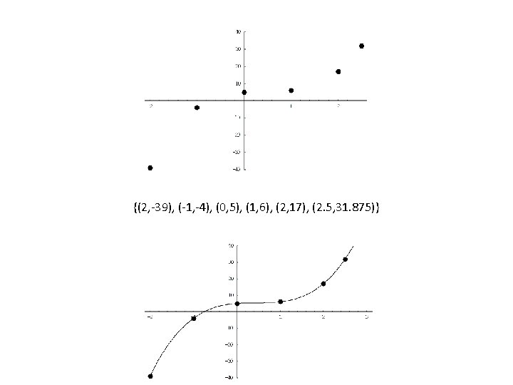
Qu. Determine f(x) as a polynomial in x for the following data Ans. x -4 -1 0 2 5 y 1245 33 5 9 1335

Numerical Integration Definite Integral The Process of Evaluating a definite integral from a set of tabulated values of f(x) is called Numerical integration If f(x) is single variable function the process is called Quadrature

Numerical integration or Quadrature • The problem of Numerical integration is to evaluate The problem arises when the integration cannot be carried out either due to fact that is not integrable or when is known only at finite number of points.

Trapezoidal rule • In numerical analysis, the trapezoidal rule (also known as the trapezoid rule or trapezium rule) is a technique for approximating the definite integral • The trapezoidal rule works by approximating the region under the graph of the function as a trapezoid and calculating its area. It follows that

The function f(x) (in blue) is approximated by a linear function (in red).

Derivation of trapezoidal and Simpson’s one third formula on integrating Newton’s Forward Difference Formula. let the interval (a, b) be divided into n equal Subintervals such that Then Newton’s forward difference interpolation formula would give us …. (1) Where and . …. (2)

Integrating of both sides of (1) between With respect to , we get and …. (3) On using (2), we obtain …. (4) Which on integration becomes …. (5)

From the equation (5), we can derive the different integration formulae by substituting We shall discuss the following particular cases. Derivation of Trapezoidal formula. Subtituting in the eq. (5), we get …. (6) Since all the other differences higher then the first Becomes zero. The equation (6) can be written as …. (7)

Similarly, we can get …. (8) …. (9) …… …… …. (10) Combining all these integrals, we get …. . (11) which is known as the Trapezoidal Rule.

Exresice Evaluate approx. by trapezoidal rule, the integral , by taking. Compute also the exact integral and find the absolute and relative error. Solution. Here The value of , and . are tabulated below: 0 0. 1 0. 2 0. 3 0. 4 0. 5 0. 6 0. 7 0. 8 0. 9 1. 0 0 0. 37 0. 68 0. 93 1. 12 1. 25 1. 32 1. 33 1. 28 1. 17 1. 0

Using Trapezoidal Rule we have Exact value Absolute Error = Exact value – Approx. value = 1 – 0. 995 = 0. 005 Relative Error = Absolute Error / Exact value = 0. 005

Exercise: 1. Evaluate by Trapezoidal rule and compare with the exact value. 2. Compute using (a) Trapezoidal rule (b) Simpson’s 1/3 rule, taking h=1. 0 and compare the results with the exact value.

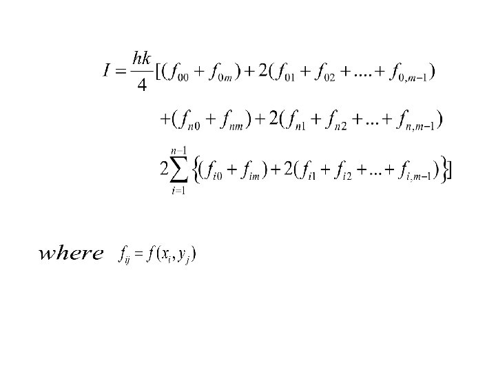
NUMERICAL DOUBLE INTEGRATION The double integral is evaluated numerically by two successive integration in x and y directions considering one at a time. Repeated application of trapezoidal rule(Simpson’s rule) yields formulae for evaluating.

Trapezoidal Rule. dividing the interval (a, b) into n equal subintervals each of length h and the interval (c, d) into m equal sub-intervals each of length k, we have: Using Trapezoidal in both directions, we get

EXERCISE: EXERCICE: Using Trapezoidal rule, evaluate taking four sub-intervals.

Solution: Taking h=k=0. 25 so that m=n=4 , we obtain

SIMPSON’S ONE-THIRD RULE: Putting n=2 in above equation and taking the curve through and as a parabola i. e. a polynomial of order second so that differences of order higher than second vanish, we get

similarly … … … , n being even. Adding all these integrals, we have when n is even

…. . (1) This is known as the Simpson’s one-third rule or simply Simpson’s rule and is most commonly used. Observations: While applying (1), the given interval must be divided into even numbers of equal sub-intervals, since we find the area of two strips at a time.

SIMPSON’S THREE-EIGHTH RULE:

EXERSICE: v EXERSICE: Evaluate By using Ø Simpson’s one-third rule Ø Simpson’s three-eighth rule

Solution: 0 1 2 3 4 5 6 1 0. 5 0. 2 0. 1 0. 0588 0. 0385 0. 027 (1) By Simpson’s one-third rule

Simpson’s three-eighth rule

NUMERICAL DOUBLE INTEGRATION Simpson’s rule: We divide the interval (a, b) into 2 n equal subintervals each of length h and the interval (c, d) into 2 m equal sub-intervals each of length k. then applying Simpson’s rule in both directions, we get

Adding all such intervals, we obtain the value of.

EXERCISE: Apply Simpson’s rule to evaluate the integral

Solutions: Taking h=0. 2 and k=0. 3 so that m=n=2, we get

EXERSICE: (1) Evaluate (h=k=0. 5). using Trapezoidal rule (2) Using Simpson’s rule, evaluate a. b. taking(h=k=0. 5)

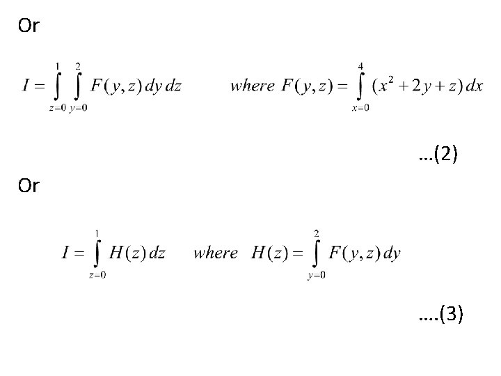
Integration with variable limits • Suppose we have to evaluate • In this case, the interval limit are of the form to. So inside integral is for y and outside one is x.

we can write where

Now the outer integral is to be evaluated using Trapezoidal or Simpson’s rule. For Trapezoidal rule (c, d) to be evaluated into n intervals at and the result may be written as Now each of are to be evaluated from by Trapezoidal rule

Example: Evaluate Solution: Let Hence . . . (1)

Now dividing (0, 1) in two subintervals at the points (0, 0. 5, 1) and using trapezoidal rule, we get Now all F(1) are obtained from (1)

Taking h=0. 105 and May construct the table as , we y 0. 5 0. 605 0. 71 z 0. 5 0. 6160 0. 7541 Hence using trapezoidal rule, we get

Evaluate: Solution: Taking and using Simpson’s rule, we get Now we go for evaluation of F(i) one by one

taking h=0. 125, we have y 0 0. 125 0. 25 z 0 0. 03125 0. 0625

Exercise: Evaluate using Trapezoidal rule Ø (Answer 3. 14) Ø (Answer -0. 747)

Exercise: Evaluate Using the Trapezoidal rule and Simpson’s rules. (take h=k=0. 5) Answer by Trapezoidal rule I=3. 0762 Answer by Simpson’s rule I=2. 9545

• Evaluation of Triple integration CONSTANT LIMIT CASE Qu. Evaluate the following using Trapezoidal Rule Solution: Let I= …(1)

• So Finally we have …. . (4) Now Apply Trapezoidal rule for Eq. (4) by dividing the interval [0, 1] in two parts as Z=(0, 0. 5, 1)

• Obtain H(0), H(0. 5) and H(1) with the help of Eq. (3) by applying Trapezoidal Rule. • Then Obtain F(i) with the help of Eq. (2) by applying Trapezoidal rule. • Compute the final Answer