Advanced and Multivariate Statistical Methods Practical Application and

Advanced and Multivariate Statistical Methods Practical Application and Interpretation Sixth Edition Craig A. Mertler and Rachel Vannatta Reinhart © 2017 Taylor & Francis

Chapter 7 Multiple Regression © 2017 Taylor & Francis

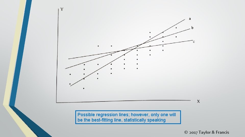
Simple Regression • Primary purpose is to develop an equation that can be used for predicting values on a DV for all members of a population o Secondary purpose is to explain causal relationships among variables (Chapter 8) • Single IV and single DV – simple linear regression, or simple regression o Capitalizes on correlation between IV and DV o Try to obtain the best-fitting line through a series of points (i. e. , bivariate scatterplot) § Line that lies closest to all points in a scatterplot; sometimes said to pass through centroid © 2017 Taylor & Francis

Possible regression lines; however, only one will be the best-fitting line, statistically speaking © 2017 Taylor & Francis

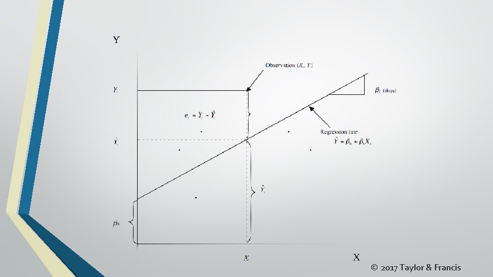
Simple Regression • To make predictions, three things about the line must be known: o Extent to which points are scattered around the line (typically indicated by degree of relationship between IV and DV – higher the relationship, better the degree of predictability) o Slope of regression line (determined by amount of change in Y that accompanies one unit change in X) o Point at which line crosses Y-axis (expected value for Y when X = 0) • Serve as basis for calculating regression equation itself © 2017 Taylor & Francis

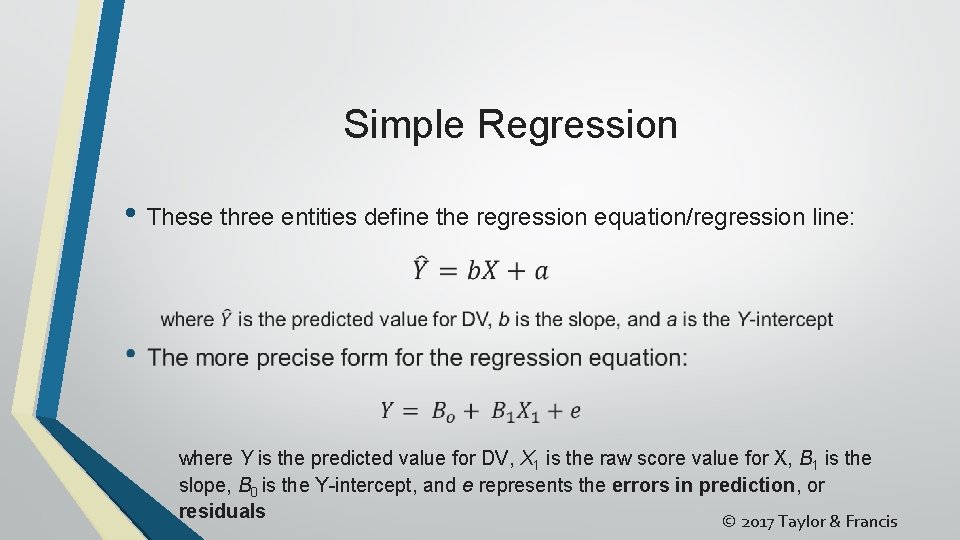
Simple Regression • These three entities define the regression equation/regression line: where Y is the predicted value for DV, X 1 is the raw score value for X, B 1 is the slope, B 0 is the Y-intercept, and e represents the errors in prediction, or residuals © 2017 Taylor & Francis

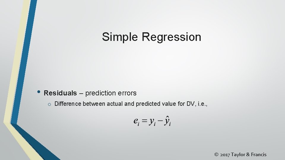
Simple Regression • Residuals – prediction errors o Difference between actual and predicted value for DV, i. e. , © 2017 Taylor & Francis

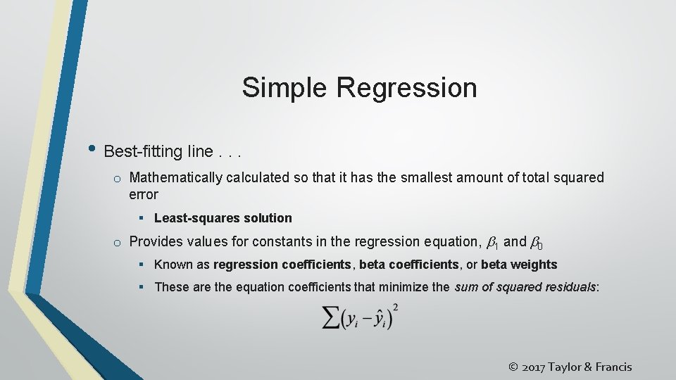
Simple Regression • Best-fitting line. . . o Mathematically calculated so that it has the smallest amount of total squared error § Least-squares solution o Provides values for constants in the regression equation, b 1 and b 0 § Known as regression coefficients, beta coefficients, or beta weights § These are the equation coefficients that minimize the sum of squared residuals: © 2017 Taylor & Francis

© 2017 Taylor & Francis

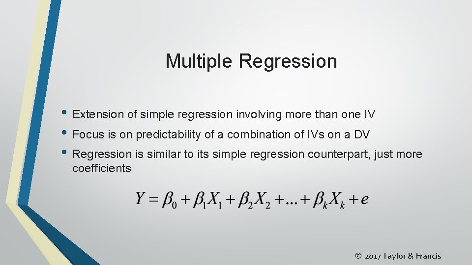
Multiple Regression • Extension of simple regression involving more than one IV • Focus is on predictability of a combination of IVs on a DV • Regression is similar to its simple regression counterpart, just more coefficients © 2017 Taylor & Francis

Multiple Regression – Unique Issues • Measures unique to MR o Linear combination of IVs that maximize correlation with DV – multiple correlation (R) § Equivalent to Pearson r between actual values and predicted values for DV o Coefficient of determination (R 2) – proportion of DV variance that can be explained by combination of IVs • Multicollinearity – problem occurring when moderate to high intercorrelations exist among IVs in same regression analysis (opposite of orthogonality) o If two variables are highly correlated, they capture much of the same information in terms of the DV © 2017 Taylor & Francis

Multiple Regression – Unique Issues o Not only does multicollinearity not help out in analysis, it can actually create problems 1) Severely limits size of R because IVs are capturing much of same variability in DV 2) Individual IV effects are confounded due to overlapping information 3) Tends to increase variance of regression coefficients, leading to less stable prediction equation o Address by examining tolerance (values <. 01 indicate problems) and variance inflation factor, or VIF (values > 10 indicate problems) o Can be dealt with by deleting problematic variable(s) or by combining variables to create a single construct (thus eliminating the repetition) © 2017 Taylor & Francis

Multiple Regression – Unique Issues • Specifying the regression model (selecting the best set of predictors) o Recall that goal should be a parsimonious solution (select IVs to give an efficient regression equation without including everything!) § Recommended ratio of participants to IVs of at least 15 to 1 © 2017 Taylor & Francis

Multiple Regression – Unique Issues • MR analysis strategies 1) Standard multiple regression – all IVs entered into analysis simultaneously; effect of each IV assessed as if it had been entered after all others (i. e. , captures only unique contribution of each IV) 2) Sequential (or hierarchical) multiple regression – IVs entered into analysis in specific order, based on previous knowledge, theory, or researcher’s plan, and assessed in terms of what each explains above and beyond all entered prior 3) Stepwise (or statistical) multiple regression – used with large set of predictors to see which make any sort of meaningful contribution © 2017 Taylor & Francis

Multiple Regression – Unique Issues 3) Stepwise (or statistical) multiple regression – approaches § Forward selection – IV with highest correlation with DV entered first, then next highest, and so on; each is assessed in terms of DR 2 (after partialing out effects of those previously entered); process continues until IVs stop making significant contributions § Stepwise selection – variation of forward selection; at each step, tests are performed to determine significance of IVs previously entered; if IV no longer makes meaningful contribution, it is dropped from the analysis § Backward deletion – initial step is to compute an equation with all predictor IVs included; each is tested as if it was entered last; if not significant, IV is removed from the analysis and subsequent equation © 2017 Taylor & Francis

Multiple Regression – Unique Issues • Cross-validation – testing prediction equation with different samples from same population o If predictive power drops off drastically for different sample, regression equation is of little overall use • Effect of outliers o MR can be very sensitive to extreme cases o Outliers should be identified and addressed prior to running regression analysis § Examine Mahalanobis distances • Multivariate multiple regression also exists (fairly analogous) © 2017 Taylor & Francis

Multiple Regression • Sample research questions – generic versions 1) Which of our predictor variables (IVs) are most influential in predicting our DV? Are there any predictor variables that do not contribute significantly to the model? 2) How reliably does the obtained prediction equation allow us to predict our DV? • Note that research questions should be worded such that they reflect the analytical approach used (i. e. , standard, sequential, or stepwise) © 2017 Taylor & Francis

Multiple Regression • Two sets of assumptions 1) About raw scale variables: § The independent variables are fixed § The independent variables are measured without error § The relationship between the independent variables and the dependent variable is linear © 2017 Taylor & Francis

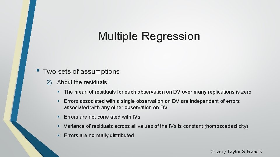
Multiple Regression • Two sets of assumptions 2) About the residuals: § The mean of residuals for each observation on DV over many replications is zero § Errors associated with a single observation on DV are independent of errors associated with any other observation on DV § Errors are not correlated with IVs § Variance of residuals across all values of the IVs is constant (homoscedasticity) § Errors are normally distributed © 2017 Taylor & Francis

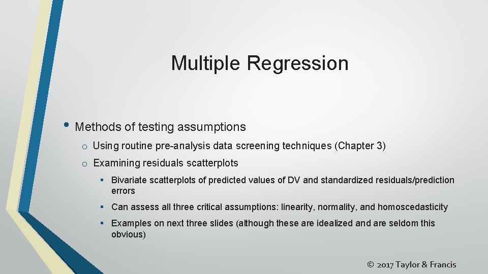
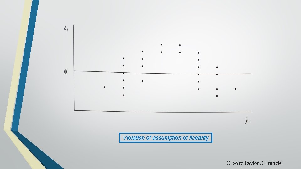
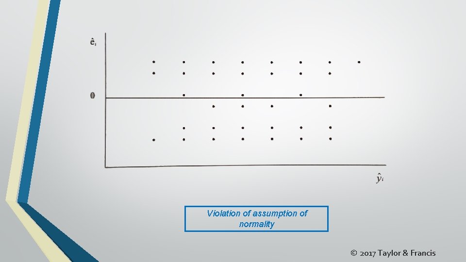
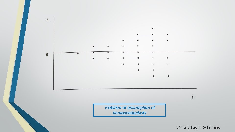
Multiple Regression • Methods of testing assumptions o Using routine pre-analysis data screening techniques (Chapter 3) o Examining residuals scatterplots § Bivariate scatterplots of predicted values of DV and standardized residuals/prediction errors § Can assess all three critical assumptions: linearity, normality, and homoscedasticity § Examples on next three slides (although these are idealized and are seldom this obvious) © 2017 Taylor & Francis

Violation of assumption of linearity © 2017 Taylor & Francis

Violation of assumption of normality © 2017 Taylor & Francis

Violation of assumption of homoscedasticity © 2017 Taylor & Francis

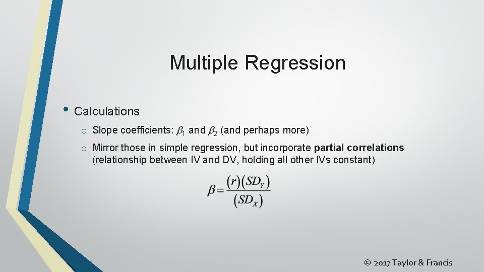
Multiple Regression • Calculations o Slope coefficients: b 1 and b 2 (and perhaps more) o Mirror those in simple regression, but incorporate partial correlations (relationship between IV and DV, holding all other IVs constant) © 2017 Taylor & Francis

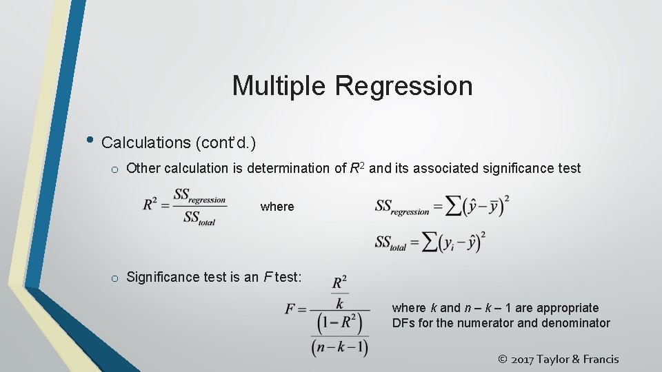
Multiple Regression • Calculations (cont’d. ) o Other calculation is determination of R 2 and its associated significance test where o Significance test is an F test: where k and n – k – 1 are appropriate DFs for the numerator and denominator © 2017 Taylor & Francis

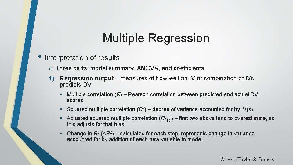
Multiple Regression • Interpretation of results o Three parts: model summary, ANOVA, and coefficients 1) Regression output – measures of how well an IV or combination of IVs predicts DV § Multiple correlation (R) – Pearson correlation between predicted and actual DV scores § Squared multiple correlation (R 2) – degree of variance accounted for by IV(s) § Adjusted squared multiple correlation (R 2 adj) – first two above tend to overestimate, so this adjusts for that bias § Change in R 2 (DR 2) – calculated for each step; represents change in variance accounted for by addition of each new variable to model © 2017 Taylor & Francis

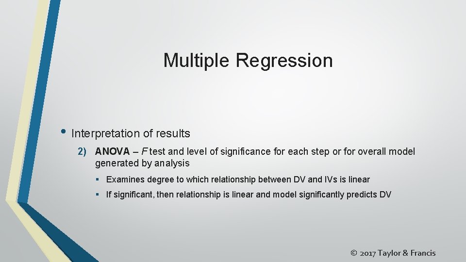
Multiple Regression • Interpretation of results 2) ANOVA – F test and level of significance for each step or for overall model generated by analysis § Examines degree to which relationship between DV and IVs is linear § If significant, then relationship is linear and model significantly predicts DV © 2017 Taylor & Francis

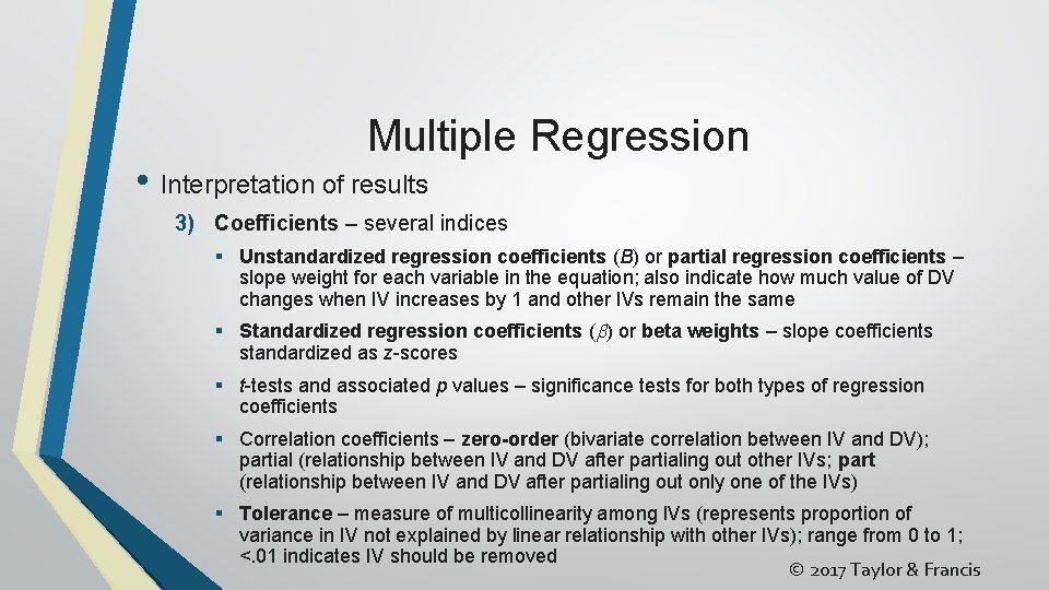
Multiple Regression • Interpretation of results 3) Coefficients – several indices § Unstandardized regression coefficients (B) or partial regression coefficients – slope weight for each variable in the equation; also indicate how much value of DV changes when IV increases by 1 and other IVs remain the same § Standardized regression coefficients (b) or beta weights – slope coefficients standardized as z-scores § t-tests and associated p values – significance tests for both types of regression coefficients § Correlation coefficients – zero-order (bivariate correlation between IV and DV); partial (relationship between IV and DV after partialing out other IVs; part (relationship between IV and DV after partialing out only one of the IVs) § Tolerance – measure of multicollinearity among IVs (represents proportion of variance in IV not explained by linear relationship with other IVs); range from 0 to 1; <. 01 indicates IV should be removed © 2017 Taylor & Francis

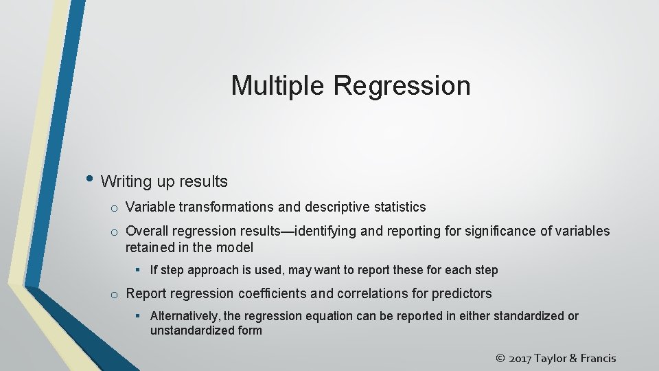
Multiple Regression • Writing up results o Variable transformations and descriptive statistics o Overall regression results—identifying and reporting for significance of variables retained in the model § If step approach is used, may want to report these for each step o Report regression coefficients and correlations for predictors § Alternatively, the regression equation can be reported in either standardized or unstandardized form © 2017 Taylor & Francis

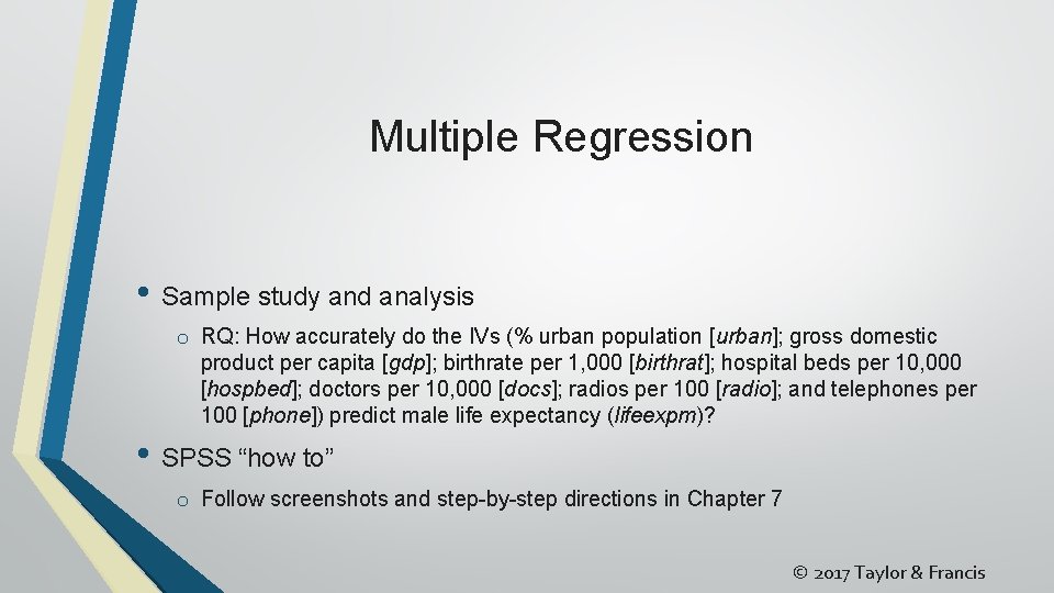
Multiple Regression • Sample study and analysis o RQ: How accurately do the IVs (% urban population [urban]; gross domestic product per capita [gdp]; birthrate per 1, 000 [birthrat]; hospital beds per 10, 000 [hospbed]; doctors per 10, 000 [docs]; radios per 100 [radio]; and telephones per 100 [phone]) predict male life expectancy (lifeexpm)? • SPSS “how to” o Follow screenshots and step-by-step directions in Chapter 7 © 2017 Taylor & Francis