Multivariate data Regression and Correlation The Scatter Plot

Multivariate data

Regression and Correlation

The Scatter Plot

Pearson’s correlation coefficient

where

Spearman’s rank correlation coefficient Where for each case i, di = ri – si = difference in the rank of xi and the rank of yi.

Simple Linear Regression Fitting straight lines to data

The Least Squares Line The Regression Line • When data is correlated it falls roughly about a straight line.

In this situation wants to: • Find the equation of the straight line through the data that yields the best fit. The equation of any straight line: is of the form: Y = a + b. X b = the slope of the line a = the intercept of the line

For any equation of a straight line Y=a +b. X The predicted value of Y when X = xi (ith case) can be computed: The error in the prediction is given by: This is called the residual for the ith case.

The residuals can be computed for each case in the sample, The residual sum of squares (RSS) is a measure of the goodness of fit of the line Y = a + b. X to the data

The optimal choice of a and b will result in the residual sum of squares attaining a minimum. If this is the case than the line: Y = a + b. X is called the Least Squares Line

Then the slope of the least squares line can be shown to be:

and the intercept of the least squares line can be shown to be:

Computing the residual sum of squares for the least squares line Once a and b have been determined this can be computed using the far right hand side. This can also be computed using the values of Sxx, Syy and Sxy. For the Least Squares Line

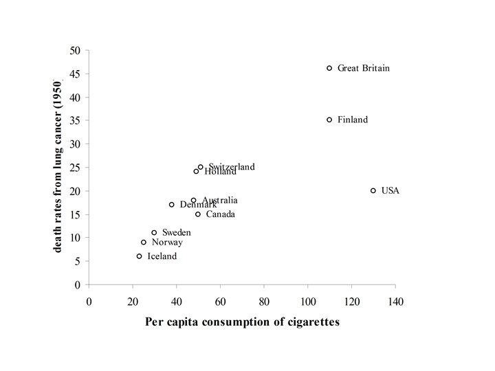
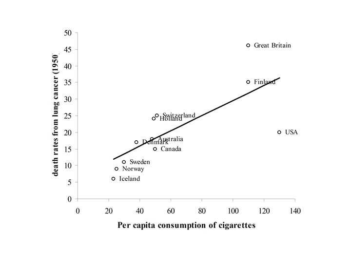
The following data showed the per capita consumption of cigarettes per month (X) in various countries in 1930, and the death rates from lung cancer for men in 1950. TABLE : Per capita consumption of cigarettes per month (Xi) in n = 11 countries in 1930, and the death rates, Yi (per 100, 000), from lung cancer for men in 1950. Country (i) Xi Yi Australia 48 18 Canada 50 15 Denmark 38 17 Finland 110 35 Great Britain 110 46 Holland 49 24 Iceland 23 6 Norway 25 9 Sweden 30 11 Switzerland 51 25 USA 130 20

Fitting the Least Squares Line

Fitting the Least Squares Line - continued First compute the following three quantities:

Computing Estimate of Slope and Intercept Computing the Residual Sum of Squares

Y = 6. 756 + (0. 228)X

Interpretation of the slope and intercept 1. Intercept – value of Y at X = 0. – Predicted death rate from lung cancer (6. 756) for men in 1950 in Counties with no smoking in 1930 (X = 0). 2. Slope – rate of increase in Y per unit increase in X. – Death rate from lung cancer for men in 1950 increases 0. 228 units for each increase of 1 cigarette per capita consumption in 1930.

Relationship between correlation and Linear Regression 1. Pearsons correlation. • Takes values between – 1 and +1

2. Least squares Line Y = a + b. X – Minimises the Residual Sum of Squares: – The Sum of Squares that measures the variability in Y that is unexplained by X. – This can also be denoted by: SSunexplained

Some other Sum of Squares: – The Sum of Squares that measures the total variability in Y (ignoring X).

– The Sum of Squares that measures the total variability in Y that is explained by X.

It can be shown: (Total variability in Y) = (variability in Y explained by X) + (variability in Y unexplained by X)

It can also be shown: = proportion variability in Y unexplained by X. = the coefficient of determination

Further: = proportion variability in Y that is unexplained by X.

Example TABLE : Per capita consumption of cigarettes per month (Xi) in n = 11 countries in 1930, and the death rates, Yi (per 100, 000), from lung cancer for men in 1950. Country (i) Xi Yi Australia 48 18 Canada 50 15 Denmark 38 17 Finland 110 35 Great Britain 110 46 Holland 49 24 Iceland 23 6 Norway 25 9 Sweden 30 11 Switzerland 51 25 USA 130 20

Computing r and r 2 54. 4% of the variability in Y (death rate due to lung Cancer (1950) is explained by X (per capita cigarette smoking in 1930)

Categorical Data Techniques for summarizing, displaying and graphing

The frequency table The bar graph Suppose we have collected data on a categorical variable X having k categories – 1, 2, … , k. To construct the frequency table we simply count for each category (i) of X, the number of cases falling in that category (fi) To plot the bar graph we simply draw a bar of height fi above each category (i) of X.

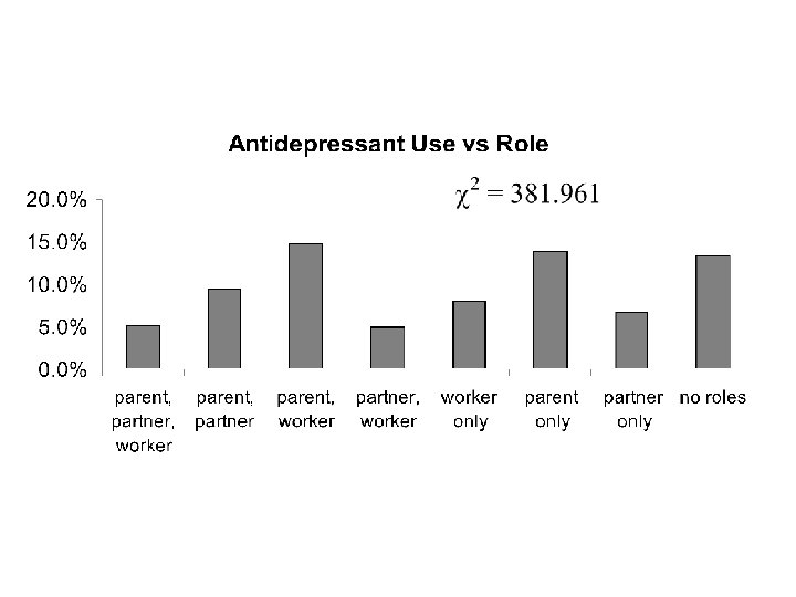
Example In this example data has been collected for n = 34, 188 subjects. • The purpose of the study was to determine the relationship between the use of Antidepressants, Mood medication, Anxiety medication, Stimulants and Sleeping pills. • In addition the study interested in examining the effects of the independent variables (gender, age, income, education and role) on both individual use of the medications and the multiple use of the medications.

The variables were: 1. Antidepressant use, 2. Mood medication use, 3. Anxiety medication use, 4. Stimulant use and 5. Sleeping pills use. 6. gender, 7. age, 8. income, 9. education and 10. Role – i. iii. iv. Parent, worker, partner v. viii. worker only Parent only Partner only No roles

Frequency Table for Age

Bar Graph for Age

Frequency Table for Role

Bar Graph for Role

The two way frequency table The c 2 statistic Techniques for examining dependence amongst two categorical variables

Situation • • We have two categorical variables R and C. The number of categories of R is r. The number of categories of C is c. We observe n subjects from the population and count xij = the number of subjects for which R = i and C = j. • R = rows, C = columns

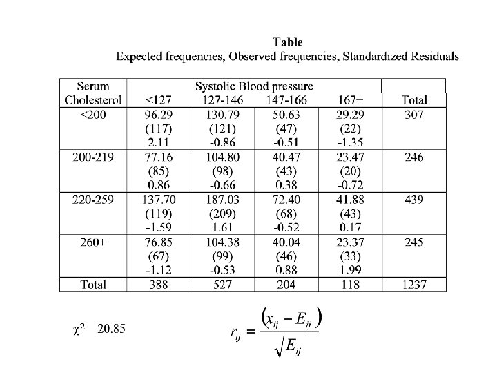
Example Both Systolic Blood pressure (C) and Serum Chlosterol (R) were meansured for a sample of n = 1237 subjects. The categories for Blood Pressure are: <126 127 -146 147 -166 167+ The categories for Chlosterol are: <200 200 -219 220 -259 260+

Table: two-way frequency Systolic Blood pressure Serum Cholesterol <127 127 -146 147 -166 167+ Total < 200 117 121 47 22 307 200 -219 85 98 43 20 246 220 -259 115 209 68 43 439 260+ 67 99 46 33 245 Total 388 527 204 118 1237

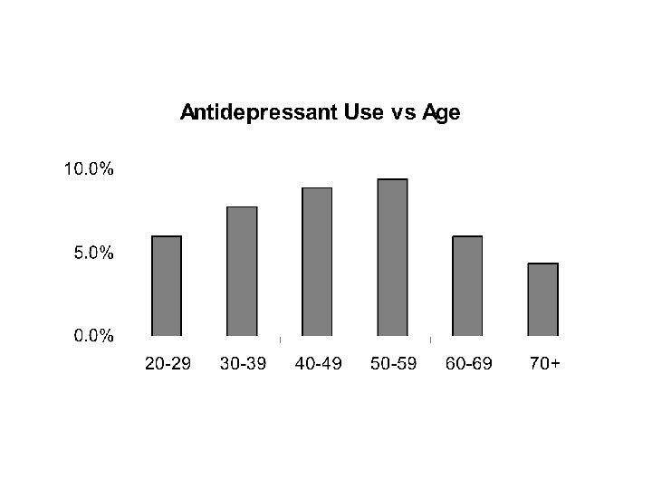
Example This comes from the drug use data. The two variables are: 1. Age (C) and 2. Antidepressant Use (R) measured for a sample of n = 33, 957 subjects.

Two-way Frequency Table Percentage antidepressant use vs Age

The c 2 statistic for measuring dependence amongst two categorical variables Define = Expected frequency in the (i, j) th cell in the case of independence.

Columns 1 2 3 4 5 Total 1 2 x 11 x 21 x 12 x 22 x 13 x 23 x 14 x 24 x 15 x 25 R 1 R 2 3 x 31 x 32 x 33 x 34 x 35 R 3 4 Total x 41 C 1 x 42 C 2 x 43 C 3 x 44 C 4 x 45 C 5 R 4 N

Columns 1 2 3 4 5 Total 1 2 E 11 E 21 E 12 E 22 E 13 E 23 E 14 E 24 E 15 E 25 R 1 R 2 3 E 31 E 32 E 33 E 34 E 35 R 3 4 Total E 41 C 1 E 42 C 2 E 43 C 3 E 44 C 4 E 45 C 5 R 4 n

Justification Proportion in column j for row i overall proportion in column j 1 2 3 4 5 Total 1 E 12 E 13 E 14 E 15 R 1 2 E 21 E 22 E 23 E 24 E 25 R 2 3 E 31 E 32 E 33 E 34 E 35 R 3 4 E 41 E 42 E 43 E 44 E 45 R 4 Total C 1 C 2 C 3 C 4 C 5 n

and Proportion in row i for column j overall proportion in row i 1 2 3 4 5 Total 1 E 12 E 13 E 14 E 15 R 1 2 E 21 E 22 E 23 E 24 E 25 R 2 3 E 31 E 32 E 33 E 34 E 35 R 3 4 E 41 E 42 E 43 E 44 E 45 R 4 Total C 1 C 2 C 3 C 4 C 5 n

The c 2 statistic Eij= Expected frequency in the (i, j) th cell in the case of independence. xij= observed frequency in the (i, j) th cell

Example: studying the relationship between Systolic Blood pressure and Serum Cholesterol In this example we are interested in whether Systolic Blood pressure and Serum Cholesterol are related or whether they are independent. Both were measured for a sample of n = 1237 cases

Observed frequencies Systolic Blood pressure Serum Cholesterol <127 127 -146 147 -166 167+ Total < 200 117 121 47 22 307 200 -219 85 98 43 20 246 220 -259 115 209 68 43 439 260+ 67 99 46 33 245 Total 388 527 204 118 1237

Expected frequencies Systolic Blood pressure Serum Cholesterol <127 127 -146 147 -166 167+ Total < 200 96. 29 130. 79 50. 63 29. 29 307 200 -219 77. 16 104. 8 40. 47 23. 47 246 220 -259 137. 70 187. 03 72. 40 41. 88 439 260+ 76. 85 104. 38 40. 04 23. 37 245 Total 388 527 204 118 1237 In the case of independence the distribution across a row is the same for each row The distribution down a column is the same for each column

Standardized residuals The c 2 statistic

Example This comes from the drug use data. The two variables are: 1. Role (C) and 2. Antidepressant Use (R) measured for a sample of n = 33, 957 subjects.

Two-way Frequency Table Percentage antidepressant use vs Role

Calculation of c 2 The Raw data Expected frequencies

The Residuals The calculation of c 2

Probability Theory Modelling random phenomena

Some counting formulae Permutations the number of ways that you can order n objects is: n! = n(n-1)(n-2)(n-3)…(3)(2)(1) Example: the number of ways you can order the three letters A, B, and C is 3! = 3(2)(1) = 6 ABC ACB BAC BCA CAB CBA

Permutations the number of ways that you can choose k objects from n objects in a specific order: Example: the number of ways you choose two letters from the four letters A, B, D, C in a specific order is

AB BA AC CA AD DA BC CB BD DB CD DC

Combinations the number of ways that you can choose k objects from n objects (order irrelevant) is:

Example: the number of ways you choose two letters from the four letters A, B, D, C {A, B} {A, C} {B, D} {C, D} {A, D} {B, C}

Example: Suppose we have a committee of 10 people and we want to choose a sub-committee of 3 people. How many ways can this be done

Example: Random sampling Suppose we have a club of N =1000 persons and we want to choose sample of k = 250 of these individuals to determine there opinion on a given issue. How many ways can this be performed? The choice of the sample is called random sampling if all of the choices has the same probability of being selected

Important Note: 0! is always defined to be 1. Also are called Binomial Coefficients

Reason: The Binomial Theorem

Binomial Coefficients can also be calculated using Pascal’s triangle 1 1 2 1 1 3 3 1 1 4 6 4 1 1 5 10 10 5 1 1 6 15 20 15 6 1

Random Variables Probability distributions

Definition: A random variable X is a number whose value is determined by the outcome of a random experiment (random phenomena)

Examples 1. A die is rolled and X = number of spots showing on the upper face. 2. Two dice are rolled and X = Total number of spots showing on the two upper faces. 3. A coin is tossed n = 100 times and X = number of times the coin toss resulted in a head. 4. A person is selected at random from a population and X = weight of that individual.

5. A sample of n = 100 individuals are selected at random from a population (i. e. all samples of n = 100 have the same probability of being selected). X = the average weight of the 100 individuals.

In all of these examples X fits the definition of a random variable, namely: – a number whose value is determined by the outcome of a random experiment (random phenomena)

Probability distribution of a Random Variable

Random variables are either • Discrete – Integer valued – The set of possible values for X are integers • Continuous – The set of possible values for X are all real numbers – Range over a continuum.

Examples • Discrete – A die is rolled and X = number of spots showing on the upper face. – Two dice are rolled and X = Total number of spots showing on the two upper faces. – A coin is tossed n = 100 times and X = number of times the coin toss resulted in a head.

Examples • Continuous – A person is selected at random from a population and X = weight of that individual. – A sample of n = 100 individuals are selected at random from a population (i. e. all samples of n = 100 have the same probability of being selected). X = the average weight of the 100 individuals.

The probability distribution of a discrete random variable is describe by its : probability function p(x) = the probability that X takes on the value x.

Examples • Discrete – A die is rolled and X = number of spots showing on the upper face. x 1 p(x) 1/6 2 1/6 3 1/6 4 1/6 5 1/6 6 1/6 – Two dice are rolled and X = Total number of spots showing on the two upper faces. x 2 3 4 5 6 7 8 9 10 11 12 p(x) 1/36 2/36 3/36 4/36 5/36 6/36 5/36 4/36 3/36 2/36 1/36

Graphs To plot a graph of p(x), draw bars of height p(x) above each value of x. Rolling a die

Rolling two dice

Note: 1. 0 p(x) 1 2. 3.

The probability distribution of a continuous random variable is described by its : probability density curve f(x).

i. e. a curve which has the following properties : • 1. f(x) is always positive. • 2. The total are under the curve f(x) is one. • 3. The area under the curve f(x) between a and b is the probability that X lies between the two values.

An Important discrete distribution The Binomial distribution Suppose we have an experiment with two outcomes – Success(S) and Failure(F). Let p denote the probability of S (Success). In this case q=1 -p denotes the probability of Failure(F). Now suppose this experiment is repeated n times independently.

Let X denote the number of successes occuring in the n repititions. Then X is a random variable. It’s possible values are 0, 1, 2, 3, 4, … , (n – 2), (n – 1), n and p(x) for any of the above values of x is given by:

X is said to have the Binomial distribution with parameters n and p.

Summary: X is said to have the Binomial distribution with parameters n and p. 1. X is the number of successes occuring in the n repititions of a Success-Failure Experiment. 2. The probability of success is p. 3.

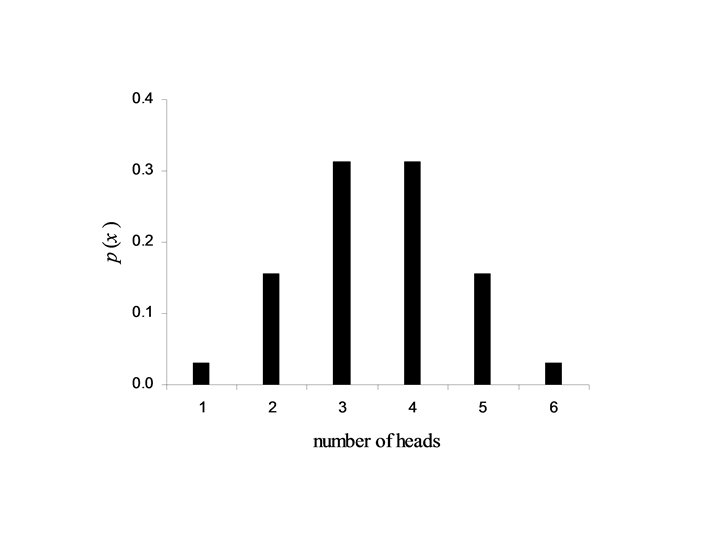
Examples: 1. A coin is tossed n = 5 times. X is the number of heads occuring in the 5 tosses of the coin. In this case p = ½ and x p(x) 0 1 2 3 4 5

Random Variables Numerical Quantities whose values are determine by the outcome of a random experiment

Discrete Random Variables Discrete Random Variable: A random variable usually assuming an integer value. • a discrete random variable assumes values that are isolated points along the real line. That is neighbouring values are not “possible values” for a discrete random variable Note: Usually associated with counting • The number of times a head occurs in 10 tosses of a coin • The number of auto accidents occurring on a weekend • The size of a family

Continuous Random Variables Continuous Random Variable: A quantitative random variable that can vary over a continuum • A continuous random variable can assume any value along a line interval, including every possible value between any two points on the line Note: Usually associated with a measurement • Blood Pressure • Weight gain • Height

Probability Distributions of a Discrete Random Variable

Probability Distribution & Function Probability Distribution: A mathematical description of how probabilities are distributed with each of the possible values of a random variable. Notes: n n The probability distribution allows one to determine probabilities of events related to the values of a random variable. The probability distribution may be presented in the form of a table, chart, formula. Probability Function: A rule that assigns probabilities to the values of the random variable

Example In baseball the number of individuals, X, on base when a home run is hit ranges in value from 0 to 3. The probability distribution is known and is given below: Note: n This chart implies the only values x takes on are 0, 1, 2, and 3. n If the random variable X is observed repeatedly the probabilities, p(x), represents the proportion times the value x appears in that sequence. 3 = = P ( the random variable X equals 2) p (2) 14

A Bar Graph

Comments: Every probability function must satisfy: 1. The probability assigned to each value of the random variable must be between 0 and 1, inclusive: 2. The sum of the probabilities assigned to all the values of the random variable must equal 1: 3.

Mean and Variance of a Discrete Probability Distribution • Describe the center and spread of a probability distribution • The mean (denoted by greek letter m (mu)), measures the centre of the distribution. • The variance (s 2) and the standard deviation (s) measure the spread of the distribution. s is the greek letter for s.

Mean of a Discrete Random Variable • The mean, m, of a discrete random variable x is found by multiplying each possible value of x by its own probability and then adding all the products together: Notes: n n n The mean is a weighted average of the values of X. The mean is the long-run average value of the random variable. The mean is centre of gravity of the probability distribution of the random variable

Variance and Standard Deviation Variance of a Discrete Random Variable: Variance, s 2, of a discrete random variable x is found by multiplying each possible value of the squared deviation from the mean, (x - m)2, by its own probability and then adding all the products together: Standard Deviation of a Discrete Random Variable: The positive square root of the variance: s = s 2

Example The number of individuals, X, on base when a home run is hit ranges in value from 0 to 3.

• Computing the mean: Note: • 0. 929 is the long-run average value of the random variable • 0. 929 is the centre of gravity value of the probability distribution of the random variable

• Computing the variance: • Computing the standard deviation:

The Binomial distribution 1. We have an experiment with two outcomes – Success(S) and Failure(F). 2. Let p denote the probability of S (Success). 3. In this case q=1 -p denotes the probability of Failure(F). 4. This experiment is repeated n times independently. 5. X denote the number of successes occuring in the n repititions.

The possible values of X are 0, 1, 2, 3, 4, … , (n – 2), (n – 1), n and p(x) for any of the above values of x is given by: X is said to have the Binomial distribution with parameters n and p.

Summary: X is said to have the Binomial distribution with parameters n and p. 1. X is the number of successes occurring in the n repetitions of a Success-Failure Experiment. 2. The probability of success is p. 3. The probability function

Example: 1. A coin is tossed n = 5 times. X is the number of heads occurring in the 5 tosses of the coin. In this case p = ½ and x p(x) 0 1 2 3 4 5

Computing the summary parameters for the distribution – m, s 2, s

• Computing the mean: • Computing the variance: • Computing the standard deviation:

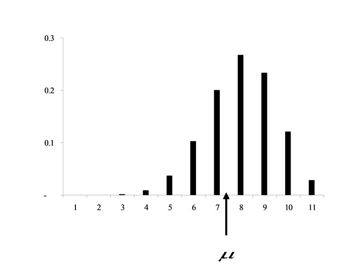
Example: • A surgeon performs a difficult operation n = 10 times. • X is the number of times that the operation is a success. • The success rate for the operation is 80%. In this case p = 0. 80 and • X has a Binomial distribution with n = 10 and p = 0. 80.

Computing p(x) for x = 1, 2, 3, … , 10

The Graph

Computing the summary parameters for the distribution – m, s 2, s

• Computing the mean: • Computing the variance: • Computing the standard deviation: