Correlation DEFINITION OF CORRELATION Correlation analysis deals with

- Slides: 30

Correlation

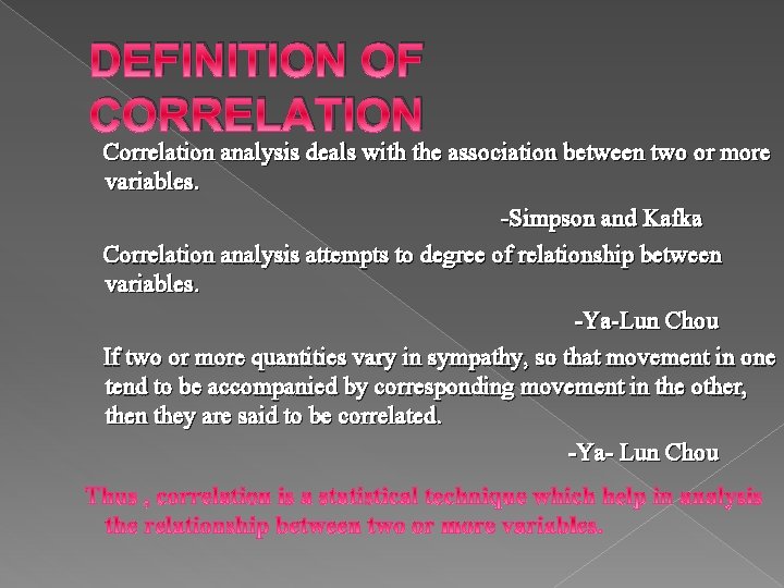
DEFINITION OF CORRELATION Correlation analysis deals with the association between two or more variables. -Simpson and Kafka Correlation analysis attempts to degree of relationship between variables. -Ya-Lun Chou If two or more quantities vary in sympathy, so that movement in one tend to be accompanied by corresponding movement in the other, then they are said to be correlated. -Ya- Lun Chou

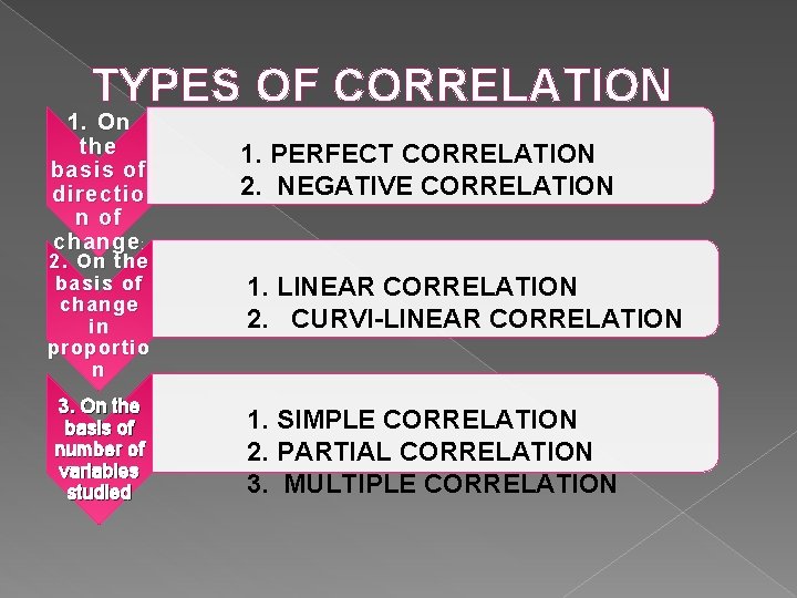
TYPES OF CORRELATION 1. On the basis of directio n of change : 2. On the basis of change in proportio n 3. On the basis of number of variables studied 1. PERFECT CORRELATION 2. NEGATIVE CORRELATION 1. LINEAR CORRELATION 2. CURVI-LINEAR CORRELATION 1. SIMPLE CORRELATION 2. PARTIAL CORRELATION 3. MULTIPLE CORRELATION

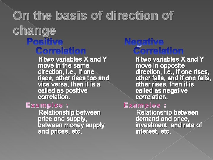
On the basis of direction of change If two variables X and Y move in the same direction, i. e. , if one rises, other rises too and vice versa, then it is a called as positive correlation. If two variables X and Y move in opposite direction, i. e. , if one rises, other falls, and if one falls, other rises, then it is called as negative correlation. Relationship between price and supply, between money supply and prices, etc. Relationship between demand price, investment and rate of interest, etc.

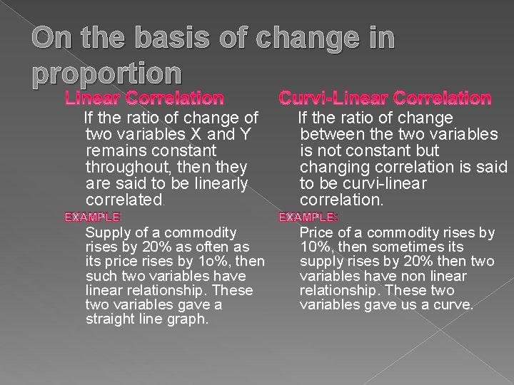
On the basis of change in proportion If the ratio of change of two variables X and Y remains constant throughout, then they are said to be linearly correlated. EXAMPLE: Supply of a commodity rises by 20% as often as its price rises by 1 o%, then such two variables have linear relationship. These two variables gave a straight line graph. If the ratio of change between the two variables is not constant but changing correlation is said to be curvi-linear correlation. EXAMPLE: Price of a commodity rises by 10%, then sometimes its supply rises by 20% then two variables have non linear relationship. These two variables gave us a curve.

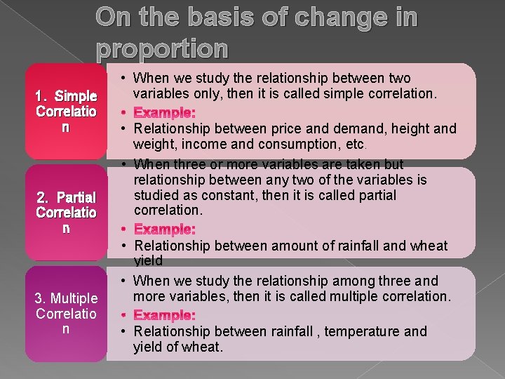
On the basis of change in proportion 1. Simple Correlatio n 2. Partial Correlatio n 3. Multiple Correlatio n • When we study the relationship between two variables only, then it is called simple correlation. • Relationship between price and demand, height and weight, income and consumption, etc. • When three or more variables are taken but relationship between any two of the variables is studied as constant, then it is called partial correlation. • Relationship between amount of rainfall and wheat yield • When we study the relationship among three and more variables, then it is called multiple correlation. • Relationship between rainfall , temperature and yield of wheat.

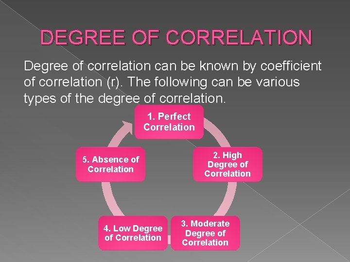
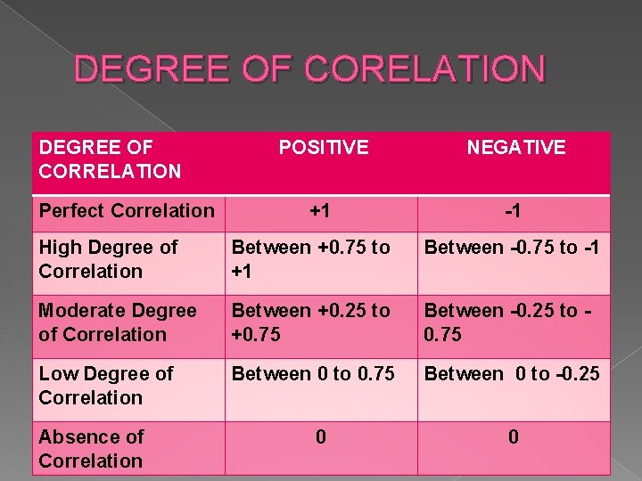
DEGREE OF CORRELATION Degree of correlation can be known by coefficient of correlation (r). The following can be various types of the degree of correlation. 1. Perfect Correlation 5. Absence of Correlation 4. Low Degree of Correlation 2. High Degree of Correlation 3. Moderate Degree of Correlation

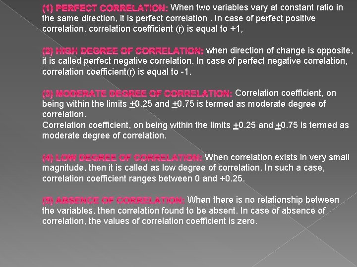
When two variables vary at constant ratio in the same direction, it is perfect correlation. In case of perfect positive correlation, correlation coefficient (r) is equal to +1, when direction of change is opposite, it is called perfect negative correlation. In case of perfect negative correlation, correlation coefficient(r) is equal to -1. Correlation coefficient, on being within the limits +0. 25 and +0. 75 is termed as moderate degree of correlation. When correlation exists in very small magnitude, then it is called as low degree of correlation. In such a case, correlation coefficient ranges between 0 and +0. 25. When there is no relationship between the variables, then correlation found to be absent. In case of absence of correlation, the values of correlation coefficient is zero.

DEGREE OF CORELATION DEGREE OF CORRELATION Perfect Correlation POSITIVE NEGATIVE +1 -1 High Degree of Correlation Between +0. 75 to +1 Between -0. 75 to -1 Moderate Degree of Correlation Between +0. 25 to +0. 75 Between -0. 25 to 0. 75 Low Degree of Correlation Between 0 to 0. 75 Between 0 to -0. 25 Absence of Correlation 0 0

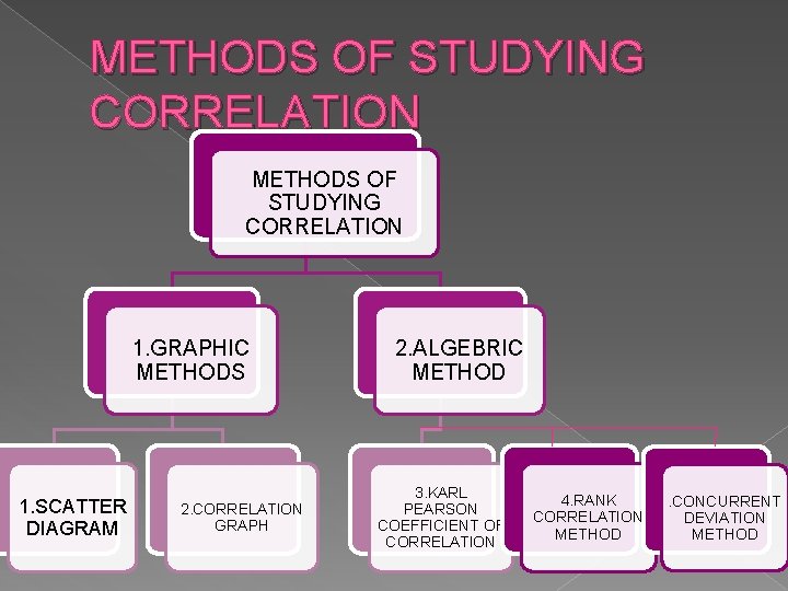
METHODS OF STUDYING CORRELATION 1. GRAPHIC METHODS 1. SCATTER DIAGRAM 2. CORRELATION GRAPH 2. ALGEBRIC METHOD 3. KARL PEARSON COEFFICIENT OF CORRELATION 4. RANK CORRELATION METHOD . CONCURRENT DEVIATION METHOD

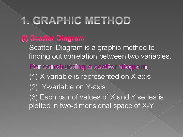
Scatter Diagram is a graphic method to finding out correlation between two variables. For constructing a scatter diagram, (1) X-variable is represented on X-axis (2) Y-variable on Y-axis. (3) Each pair of values of X and Y series is plotted in two-dimensional space of X-Y.

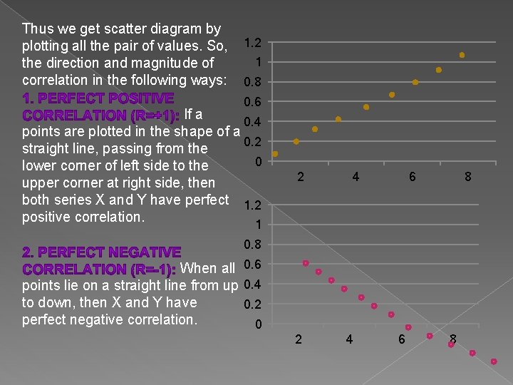
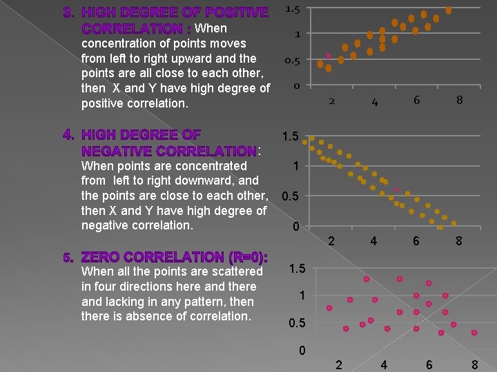
Thus we get scatter diagram by plotting all the pair of values. So, the direction and magnitude of correlation in the following ways: 1. 2 1 0. 8 0. 6 If a 0. 4 points are plotted in the shape of a 0. 2 straight line, passing from the 0 lower corner of left side to the upper corner at right side, then both series X and Y have perfect 1. 2 positive correlation. 2 4 6 8 1 0. 8 When all 0. 6 points lie on a straight line from up 0. 4 to down, then X and Y have 0. 2 perfect negative correlation. 0 2 4 6 8

1. 5 When concentration of points moves from left to right upward and the points are all close to each other, then X and Y have high degree of positive correlation. : When points are concentrated from left to right downward, and the points are close to each other, then X and Y have high degree of negative correlation. When all the points are scattered in four directions here and there and lacking in any pattern, then there is absence of correlation. 1 0. 5 0 2 4 6 8 1. 5 1 0. 5 0 2 4 6 8

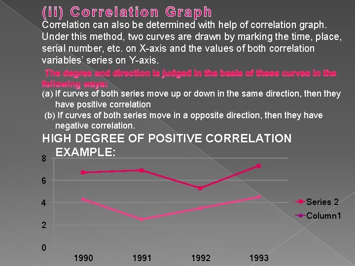
Correlation can also be determined with help of correlation graph. Under this method, two curves are drawn by marking the time, place, serial number, etc. on X-axis and the values of both correlation variables’ series on Y-axis. (a) If curves of both series move up or down in the same direction, then they have positive correlation (b) If curves of both series move in a opposite direction, then they have negative correlation. HIGH DEGREE OF POSITIVE CORRELATION EXAMPLE: 8 6 Series 2 4 Column 1 2 0 1991 1992 1993

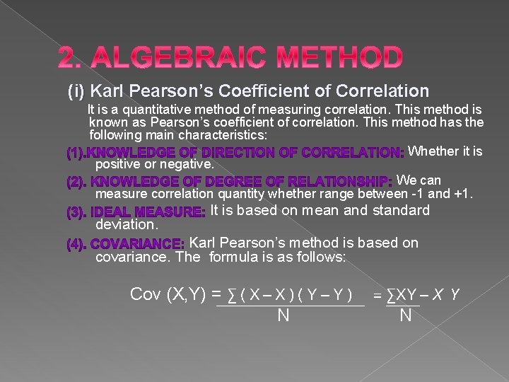
(i) Karl Pearson’s Coefficient of Correlation It is a quantitative method of measuring correlation. This method is known as Pearson’s coefficient of correlation. This method has the following main characteristics: Whether it is positive or negative. We can measure correlation quantity whether range between -1 and +1. deviation. It is based on mean and standard Karl Pearson’s method is based on covariance. The formula is as follows: Cov (X, Y) = ∑ ( X – X ) ( Y – Y ) N = ∑XY – X Y N

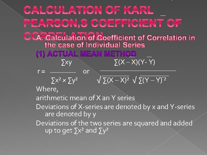
A. Calculation of Coefficient of Correlation in the case of Individual Series r= ∑xy or ∑(X – X)(Y- Y) ∑x² × ∑y² √ ∑(X – X)² √ ∑(Y – Y) ² Where, arithmetic mean of X an Y series Deviations of X-series are denoted by x and Y-series are denoted by y Deviations of the two series are squared and added up to get ∑x² and ∑y²

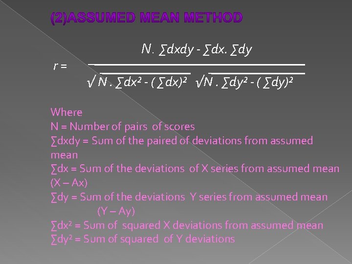
r= N. ∑dxdy - ∑dx. ∑dy √ N. ∑dx² - ( ∑dx)² √N. ∑dy² - ( ∑dy)² Where N = Number of pairs of scores ∑dxdy = Sum of the paired of deviations from assumed mean ∑dx = Sum of the deviations of X series from assumed mean (X – Ax) ∑dy = Sum of the deviations Y series from assumed mean (Y – Ay) ∑dx² = Sum of squared X deviations from assumed mean ∑dy² = Sum of squared of Y deviations

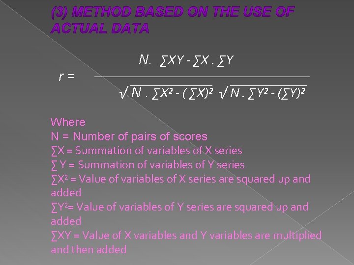
N. ∑XY - ∑X. ∑Y r= √ N. ∑X² - ( ∑X)² √ N. ∑Y² - (∑Y)² Where N = Number of pairs of scores ∑X = Summation of variables of X series ∑ Y = Summation of variables of Y series ∑X² = Value of variables of X series are squared up and added ∑Y²= Value of variables of Y series are squared up and added ∑XY = Value of X variables and Y variables are multiplied and then added

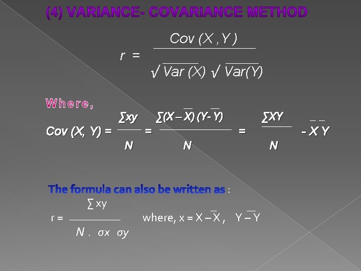
Cov (X , Y ) r = √ Var (X) √ Var(Y) ∑xy Cov (X, Y) = r= N ∑ xy N. σx σy ∑(X – X) (Y- Y) = ∑XY = N : where, x = X – X , Y – Y N -XY

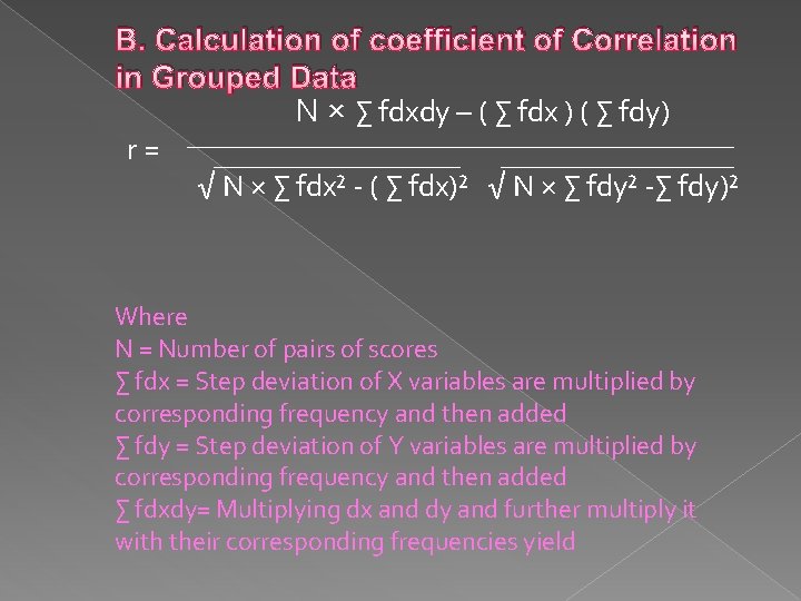
B. Calculation of coefficient of Correlation in Grouped Data N × ∑ fdxdy – ( ∑ fdx ) ( ∑ fdy) r= √ N × ∑ fdx² - ( ∑ fdx)² √ N × ∑ fdy² -∑ fdy)² Where N = Number of pairs of scores ∑ fdx = Step deviation of X variables are multiplied by corresponding frequency and then added ∑ fdy = Step deviation of Y variables are multiplied by corresponding frequency and then added ∑ fdxdy= Multiplying dx and dy and further multiply it with their corresponding frequencies yield

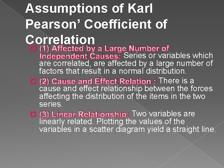
Assumptions of Karl Pearson’ Coefficient of Correlation � (1) Affected by a Large Number of Independent Causes: Series or variables which are correlated, are affected by a large number of factors that result in a normal distribution. � (2) Cause and Effect Relation : There is a cause and effect relationship between the forces affecting the distribution of the items in the two series. � (3) Linear Relationship: Two variables are linearly related. Plotting the values of the variables in a scatter diagram yield a straight line.

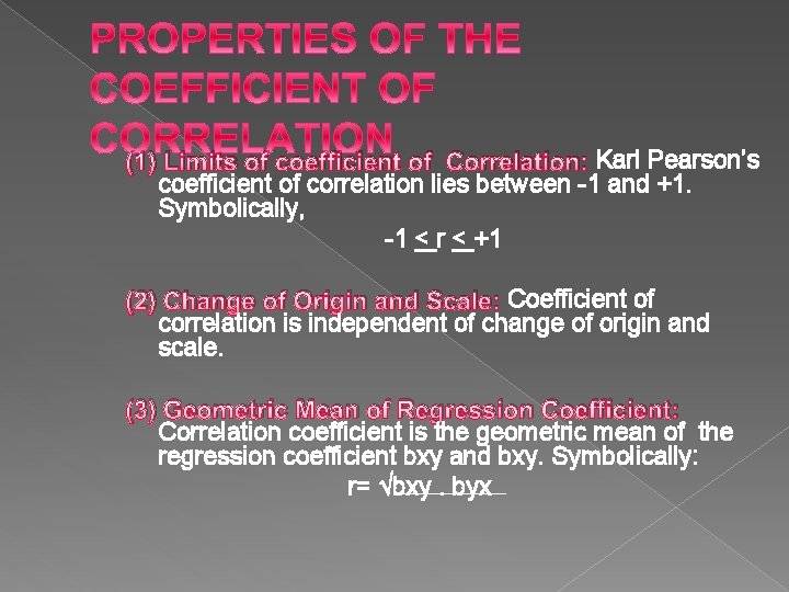
(1) Limits of coefficient of Correlation: Karl Pearson’s coefficient of correlation lies between -1 and +1. Symbolically, -1 < r < +1 (2) Change of Origin and Scale: Coefficient of correlation is independent of change of origin and scale. (3) Geometric Mean of Regression Coefficient: Correlation coefficient is the geometric mean of the regression coefficient bxy and bxy. Symbolically: r= √bxy. byx

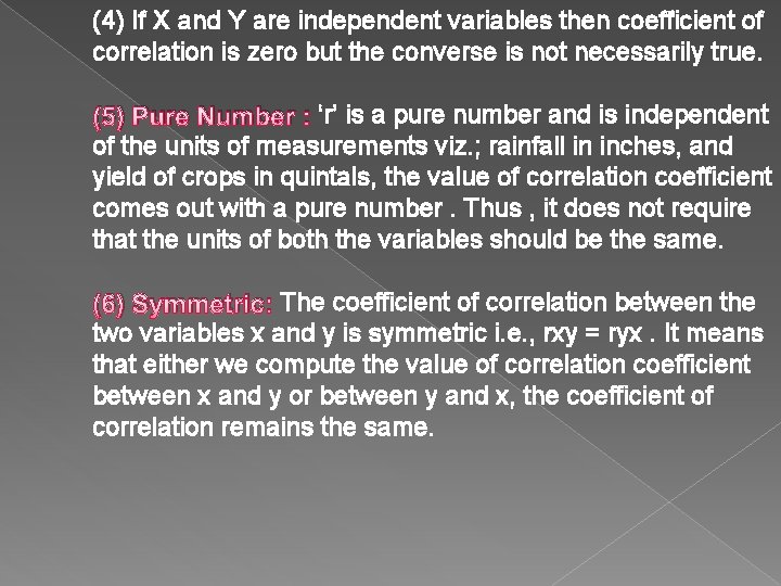
(4) If X and Y are independent variables then coefficient of correlation is zero but the converse is not necessarily true. (5) Pure Number : ‘r’ is a pure number and is independent of the units of measurements viz. ; rainfall in inches, and yield of crops in quintals, the value of correlation coefficient comes out with a pure number. Thus , it does not require that the units of both the variables should be the same. (6) Symmetric: The coefficient of correlation between the two variables x and y is symmetric i. e. , rxy = ryx. It means that either we compute the value of correlation coefficient between x and y or between y and x, the coefficient of correlation remains the same.

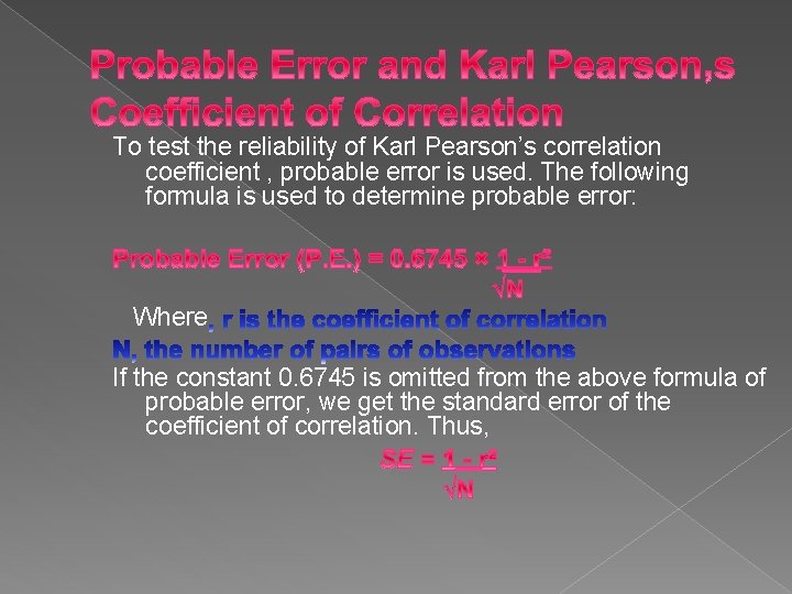
To test the reliability of Karl Pearson’s correlation coefficient , probable error is used. The following formula is used to determine probable error: Where If the constant 0. 6745 is omitted from the above formula of probable error, we get the standard error of the coefficient of correlation. Thus,

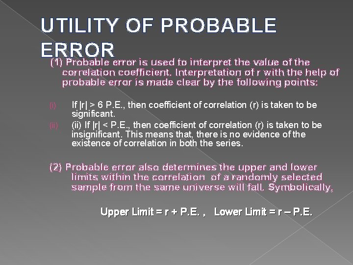
UTILITY OF PROBABLE ERROR (1) Probable error is used to interpret the value of the correlation coefficient. Interpretation of r with the help of probable error is made clear by the following points: (i) (ii) If |r| > 6 P. E. , then coefficient of correlation (r) is taken to be significant. (ii) If |r| < P. E. , then coefficient of correlation (r) is taken to be insignificant. This means that, there is no evidence of the existence of correlation in both the series. (2) Probable error also determines the upper and lower limits within the correlation of a randomly selected sample from the same universe will fall. Symbolically, Upper Limit = r + P. E. , Lower Limit = r – P. E.

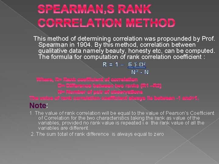
This method of determining correlation was propounded by Prof. Spearman in 1904. By this method, correlation between qualitative data namely beauty, honesty etc, can be computed. The formula for computation of rank correlation coefficient : R = 1 – 6 ∑ D² N³ - N Note: 1. The value of rank correlation will be equal to the value of Pearson’s Coefficient of Correlation for the two characteristics taking the rank as value of the variables, provided no rank value is repeated i. e. the rank value of all the variables are different. 2. The sum total of rank difference is always equal to zero

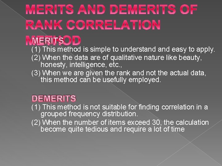
MERITS (1) This method is simple to understand easy to apply. (2) When the data are of qualitative nature like beauty, honesty, intelligence, etc. , (3) When we are given the rank and not the actual data, this method can be usefully employed. DEMERITS (1) This method is not suitable for finding correlation in a grouped frequency distribution. (2) When the number of items exceed 30, the calculation become quite tedious and require a lot of time

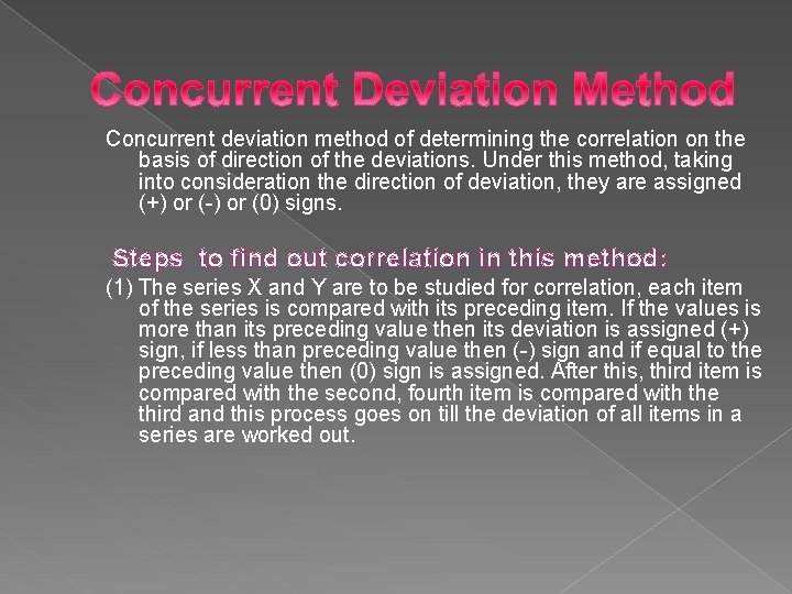
Concurrent deviation method of determining the correlation on the basis of direction of the deviations. Under this method, taking into consideration the direction of deviation, they are assigned (+) or (-) or (0) signs. Steps to find out correlation in this method: (1) The series X and Y are to be studied for correlation, each item of the series is compared with its preceding item. If the values is more than its preceding value then its deviation is assigned (+) sign, if less than preceding value then (-) sign and if equal to the preceding value then (0) sign is assigned. After this, third item is compared with the second, fourth item is compared with the third and this process goes on till the deviation of all items in a series are worked out.

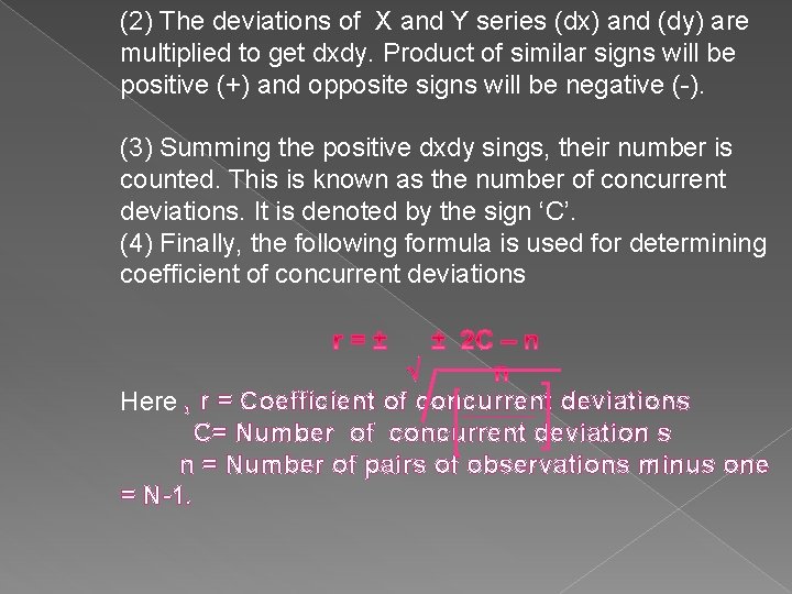
(2) The deviations of X and Y series (dx) and (dy) are multiplied to get dxdy. Product of similar signs will be positive (+) and opposite signs will be negative (-). (3) Summing the positive dxdy sings, their number is counted. This is known as the number of concurrent deviations. It is denoted by the sign ‘C’. (4) Finally, the following formula is used for determining coefficient of concurrent deviations Here , r = Coefficient of concurrent deviations C= Number of concurrent deviation s n = Number of pairs of observations minus one = N-1.
