Multivariate Analysis Machine Learning in HEP IN 2

Multivariate Analysis (Machine Learning) … in HEP IN 2 P 3 School of Statistics 2016 Helge Voss MAX-PLANCK-INSTITUT FÜR KERNPHYSIK IN HEIDELBERG Helge Voss SOS 2016, Autrans France, Multivariate Analysis – Machine Learning 1

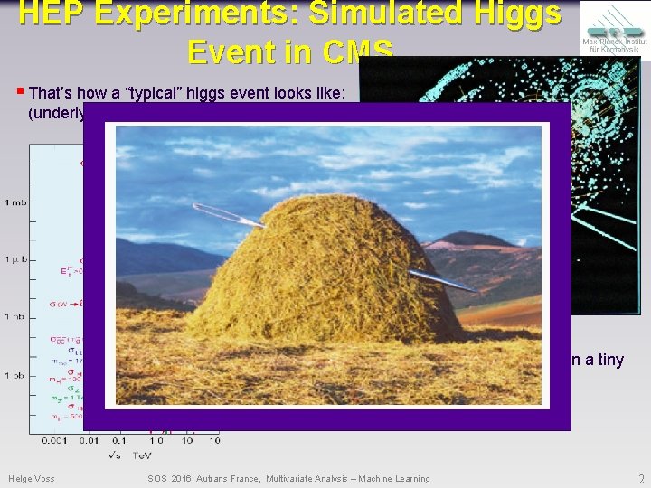
HEP Experiments: Simulated Higgs Event in CMS § That’s how a “typical” higgs event looks like: (underlying ~23 ‘minimum bias’ events) § And not only this: These event happen only in a tiny fraction of the collisions O(10 -11) Helge Voss SOS 2016, Autrans France, Multivariate Analysis – Machine Learning 2

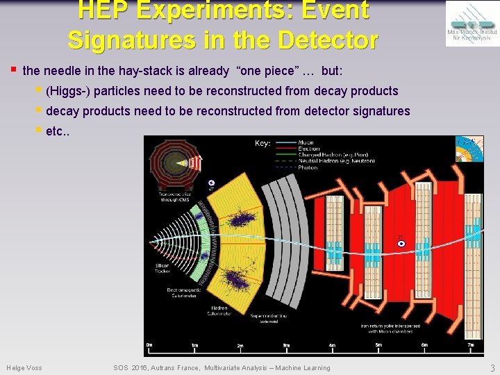
HEP Experiments: Event Signatures in the Detector § the needle in the hay-stack is already “one piece” … but: § (Higgs-) particles need to be reconstructed from decay products § decay products need to be reconstructed from detector signatures § etc. . Helge Voss SOS 2016, Autrans France, Multivariate Analysis – Machine Learning 3

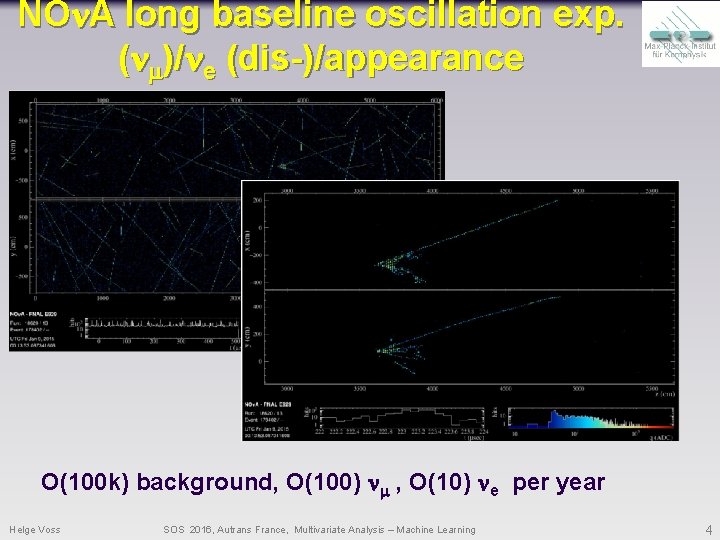
NOn. A long baseline oscillation exp. (nm)/ne (dis-)/appearance O(100 k) background, O(100) nm , O(10) ne per year Helge Voss SOS 2016, Autrans France, Multivariate Analysis – Machine Learning 4

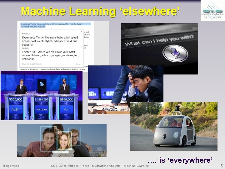
Machine Learning ‘elsewhere’ Helge Voss …. is ‘everywhere’ SOS 2016, Autrans France, Multivariate Analysis – Machine Learning 5

Outline § What is: Machine Learning (ML) & Multivariate Analysis/Technique (MVA) § Basics (classification, regression) § ROC-curve § generative vs predictive models § MVA/ML algorithms § Naïve Basian, KNN, § Linear discriminators, SVM § model fitting – gradient decent and loss function § General comments about MVAs § BDT (Yann Coadou) this afternoon) § Neural Networks (tomorrow) Helge Voss SOS 2016, Autrans France, Multivariate Analysis – Machine Learning 6

What is Machine Learning § “[Machine Learning is the] field of study that gives computers the ability to learn without being explicitly programmed. ” Arthur Samuel (1959) § “A computer program is said to learn from experience E with respect to some task T and some performance measure P, if its performance on T, as measured by P, improves with experience E. ” Tom Mitchell, Carnegie Mellon University (1997) I suggest: forget about ‘fancy definitions’: ‘understanding/modeling your data’ … and if you cannot do it in multi-dimensions on “analytic first principles” let the computer help Helge Voss SOS 2016, Autrans France, Multivariate Analysis – Machine Learning 7

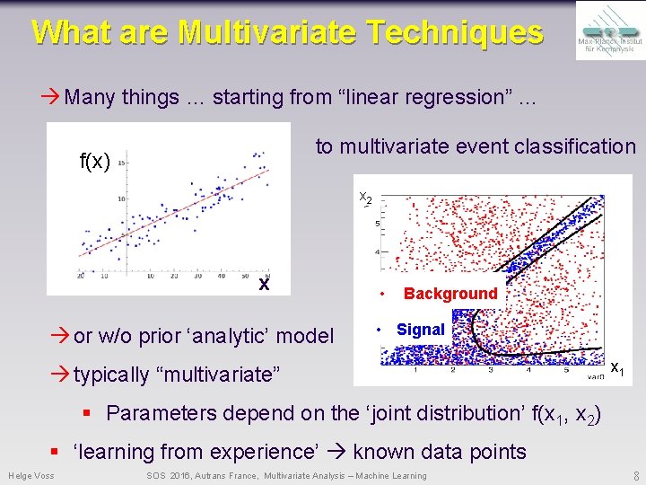
What are Multivariate Techniques Many things … starting from “linear regression” … to multivariate event classification f(x) x 2 x or w/o prior ‘analytic’ model • Background • Signal typically “multivariate” x 1 § Parameters depend on the ‘joint distribution’ f(x 1, x 2) § ‘learning from experience’ known data points Helge Voss SOS 2016, Autrans France, Multivariate Analysis – Machine Learning 8

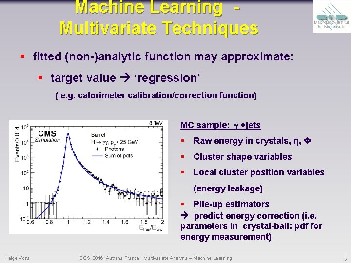
Machine Learning Multivariate Techniques § fitted (non-)analytic function may approximate: § target value ‘regression’ ( e. g. calorimeter calibration/correction function) MC sample: g +jets § Raw energy in crystals, η, Φ § Cluster shape variables § Local cluster position variables (energy leakage) § Pile-up estimators predict energy correction (i. e. parameters in crystal-ball: pdf for energy measurement) Helge Voss SOS 2016, Autrans France, Multivariate Analysis – Machine Learning 9

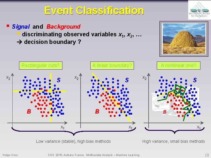
Event Classification § Signal and Background § discriminating observed variables x 1, x 2, … decision boundary ? Rectangular cuts? x 2 A linear boundary? x 2 S B x 1 Low variance (stable), high bias methods Helge Voss A nonlinear one? SOS 2016, Autrans France, Multivariate Analysis – Machine Learning x 1 High variance, small bias methods 10

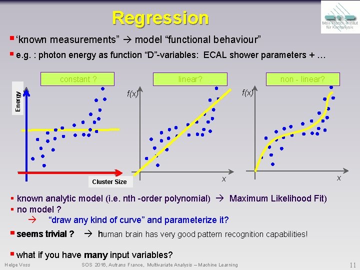
Regression § ‘known measurements” model “functional behaviour” § e. g. : photon energy as function “D”-variables: constant ? ECAL shower parameters + … linear? non - linear? f(x) Energy f(x) x Size Cluster x x § known analytic model (i. e. nth -order polynomial) Maximum Likelihood Fit) § no model ? “draw any kind of curve” and parameterize it? § seems trivial ? human brain has very good pattern recognition capabilities! § what if you have many input variables? Helge Voss SOS 2016, Autrans France, Multivariate Analysis – Machine Learning 11

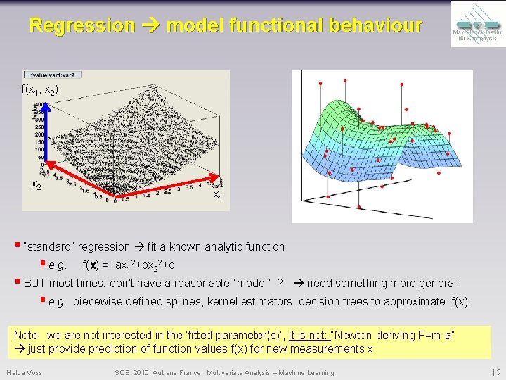
Regression model functional behaviour f(x 1, x 2) x 2 x 1 § “standard” regression fit a known analytic function § e. g. f(x) = ax 12+bx 22+c § BUT most times: don’t have a reasonable “model” ? need something more general: § e. g. piecewise defined splines, kernel estimators, decision trees to approximate f(x) Note: we are not interested in the ‘fitted parameter(s)’, it is not: “Newton deriving F=m·a” just provide prediction of function values f(x) for new measurements x Helge Voss SOS 2016, Autrans France, Multivariate Analysis – Machine Learning 12

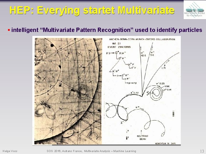
HEP: Everying startet Multivariate § intelligent “Multivariate Pattern Recognition” used to identify particles Helge Voss SOS 2016, Autrans France, Multivariate Analysis – Machine Learning 13

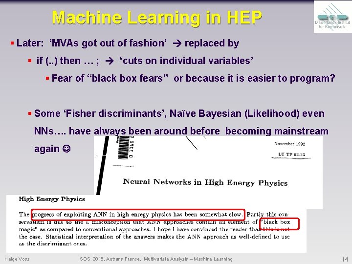
Machine Learning in HEP § Later: ‘MVAs got out of fashion’ replaced by § if (. . ) then … ; ‘cuts on individual variables’ § Fear of “black box fears” or because it is easier to program? § Some ‘Fisher discriminants’, Naïve Bayesian (Likelihood) even NNs…. have always been around before becoming mainstream again Helge Voss SOS 2016, Autrans France, Multivariate Analysis – Machine Learning 14

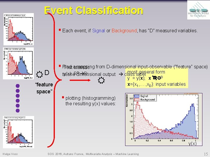
Event Classification § Each event, if Signal or Background, has “D” measured variables. D “feature space” § Find mapping from D-dimensional input-observable (”feature” space) Test astatistic: most general form D R: y(x): to one. Rdimensional output class label y = y(x); x D x={x 1, …. , x. D}: input variables § plotting (histogramming) the resulting y(x) values: y(x) Helge Voss SOS 2016, Autrans France, Multivariate Analysis – Machine Learning 15

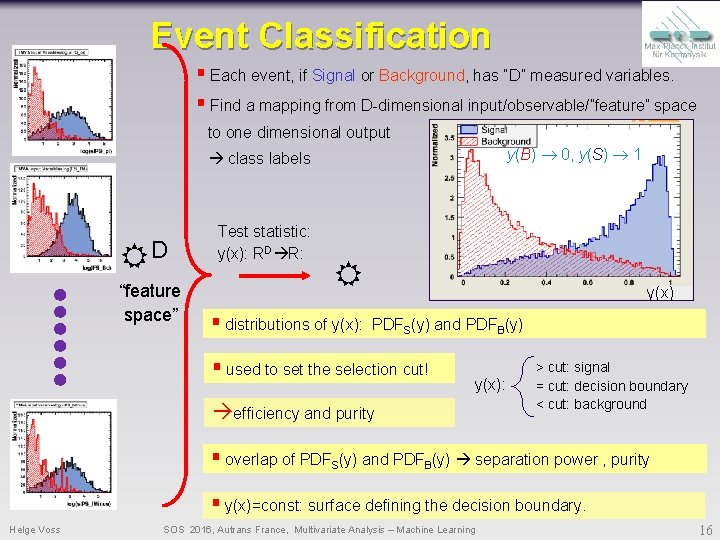
Event Classification § Each event, if Signal or Background, has “D” measured variables. § Find a mapping from D-dimensional input/observable/”feature” space to one dimensional output y(B) 0, y(S) 1 class labels D “feature space” Test statistic: y(x): RD R: § distributions of y(x): y(x) PDFS(y) and PDFB(y) § used to set the selection cut! y(x): efficiency and purity > cut: signal = cut: decision boundary < cut: background § overlap of PDFS(y) and PDFB(y) separation power , purity § y(x)=const: surface defining the decision boundary. Helge Voss SOS 2016, Autrans France, Multivariate Analysis – Machine Learning 16

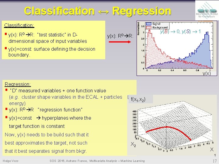
Classification ↔ Regression Classification: § y(x): RD R: “test statistic” in Ddimensional space of input variables y(x): RD R: y(B) 0, y(S) 1 § y(x)=const: surface defining the decision boundary. y(x) Regression: § “D” measured variables + one function value (e. g. cluster shape variables in the ECAL + particles energy) § y(x): RD R “regression function” § y(x)=const f(x 1, x 2) hyperplanes where the target function is constant Now, y(x) needs to be build such that it best approximates the target, not such X 2 that it best separates signal from bkgr. Helge Voss SOS 2016, Autrans France, Multivariate Analysis – Machine Learning X 1 17

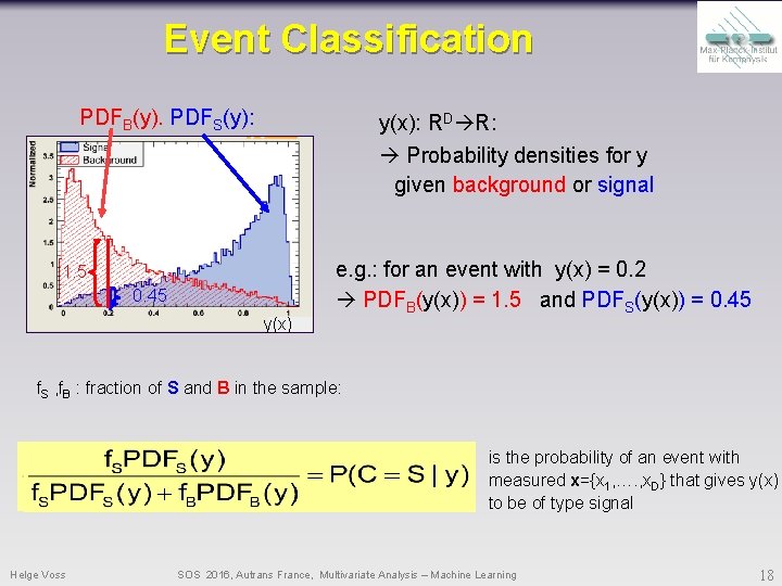
Event Classification PDFB(y). PDFS(y): y(x): RD R: Probability densities for y given background or signal 1. 5 0. 45 y(x) e. g. : for an event with y(x) = 0. 2 PDFB(y(x)) = 1. 5 and PDFS(y(x)) = 0. 45 f. S , f. B : fraction of S and B in the sample: is the probability of an event with measured x={x 1, …. , x. D} that gives y(x) to be of type signal Helge Voss SOS 2016, Autrans France, Multivariate Analysis – Machine Learning 18

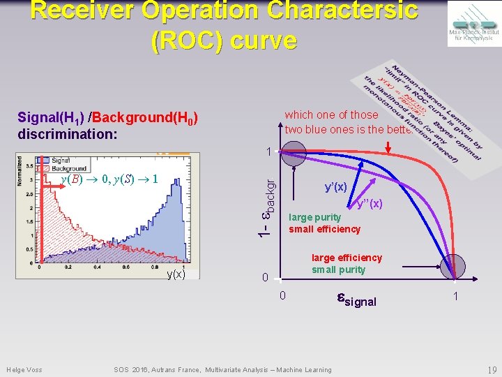
Receiver Operation Charactersic (ROC) curve which one of those two blue ones is the better? ? Signal(H 1) /Background(H 0) discrimination: 1 1 - ebackgr. y(B) 0, y(S) 1 y(x) y’’(x) large purity small efficiency large efficiency small purity 0 0 Helge Voss SOS 2016, Autrans France, Multivariate Analysis – Machine Learning esignal 1 19

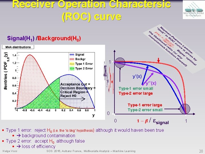
Receiver Operation Charactersic (ROC) curve Signal(H 1) /Background(H 0) 1 y’(x) y’’(x) Type-1 error small Type-2 error large Type-1 error large Type-2 error small 0 0 § Type 1 error: reject H 0 (i. e. the ‘is bkg’ hypothesis) although it would haven been true § background contamination § Type 2 error: accept H 0 although false § loss of efficiency Helge Voss SOS 2016, Autrans France, Multivariate Analysis – Machine Learning 1 20

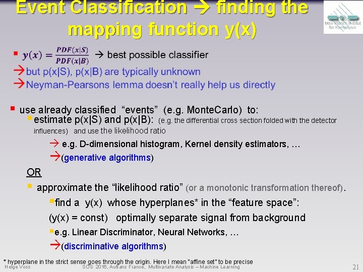
Event Classification finding the mapping function y(x) § use already classified “events” (e. g. Monte. Carlo) to: § estimate p(x|S) and p(x|B): (e. g. the differential cross section folded with the detector influences) and use the likelihood ratio e. g. D-dimensional histogram, Kernel density estimators, … (generative algorithms) OR § approximate the “likelihood ratio” (or a monotonic transformation thereof). §find a y(x) whose hyperplanes* in the “feature space”: (y(x) = const) optimally separate signal from background §e. g. Linear Discriminator, Neural Networks, … (discriminative algorithms) * hyperplane in the strict sense goes through the origin. Here I mean “affine set” to be precise Helge Voss SOS 2016, Autrans France, Multivariate Analysis – Machine Learning 21

Machine Learning Categories supervised: value) - training “events” with known type (i. e. Signal or Backgr, target un-supervised: - no prior notion of “Signal” or “Background” - cluster analysis: if different “groups” are found class labels - principal component analysis: find basis in observable space with biggest hierarchical differences in the variance infer something about underlying substructure reinforcement-learning: - learn from “success” or “failure” of some “action policy” (i. e. a robot achieves his goal or does not / falls or does not fall/ wins looses the game) or This lecture: supervised learning Helge Voss SOS 2016, Autrans France, Multivariate Analysis – Machine Learning 22

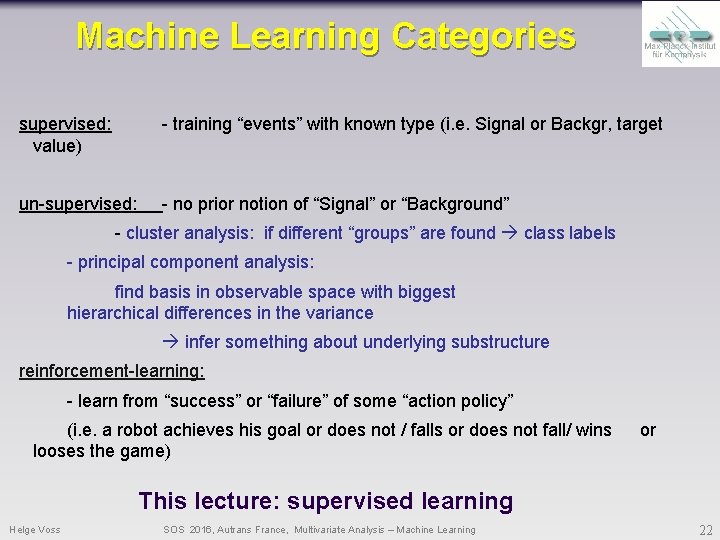
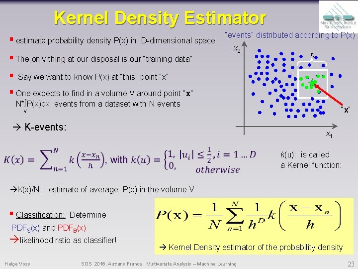
Kernel Density Estimator § estimate probability density P(x) in D-dimensional space: § The only thing at our disposal is our “training data” “events” distributed according to P(x) x 2 h § Say we want to know P(x) at “this” point “x” § One expects to find in a volume V around point “x” N*∫P(x)dx events from a dataset with N events “x” V K-events: x 1 k(u): is called a Kernel function: K(x)/N: estimate of average P(x) in the volume V § Classification: Determine PDFS(x) and PDFB(x) likelihood ratio as classifier! Helge Voss Kernel Density estimator of the probability density SOS 2016, Autrans France, Multivariate Analysis – Machine Learning 23

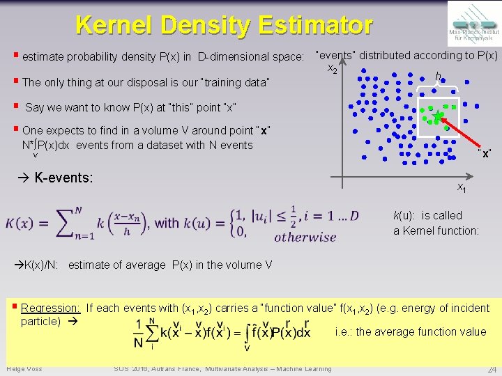
Kernel Density Estimator § estimate probability density P(x) in D-dimensional space: “events” distributed according to P(x) x 2 h § The only thing at our disposal is our “training data” § Say we want to know P(x) at “this” point “x” § One expects to find in a volume V around point “x” N*∫P(x)dx events from a dataset with N events “x” V K-events: x 1 k(u): is called a Kernel function: K(x)/N: estimate of average P(x) in the volume V § Regression: particle) Helge Voss If each events with (x 1, x 2) carries a “function value” f(x 1, x 2) (e. g. energy of incident i. e. : the average function value SOS 2016, Autrans France, Multivariate Analysis – Machine Learning 24

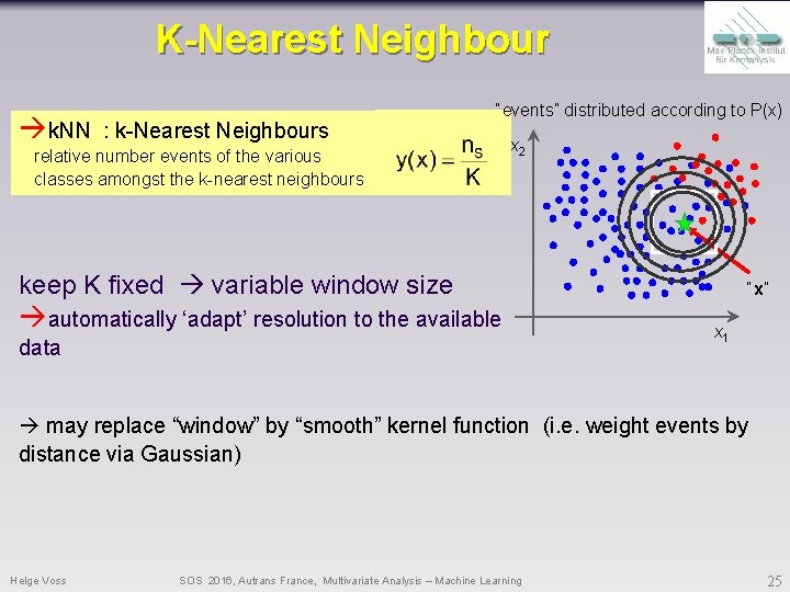
K-Nearest Neighbour k. NN : k-Nearest Neighbours “events” distributed according to P(x) relative number events of the various classes amongst the k-nearest neighbours x 2 keep K fixed variable window size automatically ‘adapt’ resolution to the available data “x” x 1 may replace “window” by “smooth” kernel function (i. e. weight events by distance via Gaussian) Helge Voss SOS 2016, Autrans France, Multivariate Analysis – Machine Learning 25

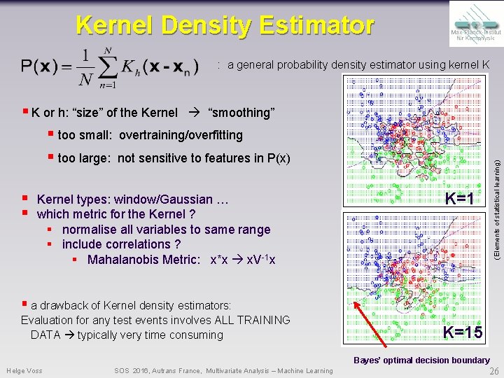
Kernel Density Estimator : a general probability density estimator using kernel K § § Kernel types: window/Gaussian … which metric for the Kernel ? § normalise all variables to same range § include correlations ? § Mahalanobis Metric: x*x x. V-1 x (Elements of statistical learning) § K or h: “size” of the Kernel “smoothing” § too small: overtraining/overfitting § too large: not sensitive to features in P(x) K=1 § a drawback of Kernel density estimators: Evaluation for any test events involves ALL TRAINING DATA typically very time consuming K=15 Bayes’ optimal decision boundary Helge Voss SOS 2016, Autrans France, Multivariate Analysis – Machine Learning 26

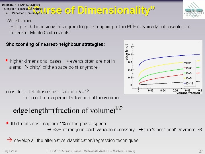
Bellman, R. (1961), Adaptive Control Processes: A Guided Tour, Princeton University Press. “Curse of Dimensionality” We all know: Filling a D-dimensional histogram to get a mapping of the PDF is typically unfeasable due to lack of Monte Carlo events. Shortcoming of nearest-neighbour strategies: § higher dimensional cases K-events often are not in a small “vicinity” of the space point anymore: consider: total phase space volume V=1 D for a cube of a particular fraction of the volume: § 10 dimensions: capture 1% of the phase space 63% of range in each variable necessary that’s not “local” anymore. . develop all the alternative classification/regression techniques Helge Voss SOS 2016, Autrans France, Multivariate Analysis – Machine Learning 27

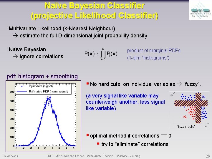
Naïve Bayesian Classifier (projective Likelihood Classifier) Multivariate Likelihood (k-Nearest Neighbour) estimate the full D-dimensional joint probability density Naïve Bayesian ignore correlations pdf: histogram + smoothing product of marginal PDFs (1 -dim “histograms”) § No hard cuts on individual variables “fuzzy”, (a very signal like variable may counterweigh another, less signal like variable) “fuzzy cuts” § optimal method if correlations == 0 § try to “eliminate” correlations Helge Voss SOS 2016, Autrans France, Multivariate Analysis – Machine Learning 28

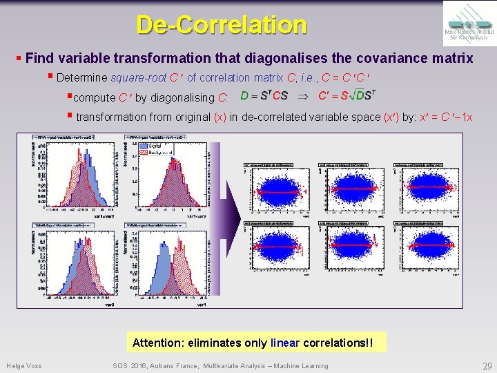
De-Correlation § Find variable transformation that diagonalises the covariance matrix § Determine square-root C of correlation matrix C, i. e. , C = C C §compute C by diagonalising C: § transformation from original (x) in de-correlated variable space (x ) by: x = C 1 x Attention: eliminates only linear correlations!! Helge Voss SOS 2016, Autrans France, Multivariate Analysis – Machine Learning 29

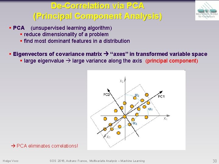
De-Correlation via PCA (Principal Component Analysis) § PCA (unsupervised learning algorithm) § reduce dimensionality of a problem § find most dominant features in a distribution § Eigenvectors of covariance matrix “axes” in transformed variable space § large eigenvalue large variance along the axis (principal component) PCA eliminates correlations! Helge Voss SOS 2016, Autrans France, Multivariate Analysis – Machine Learning 30

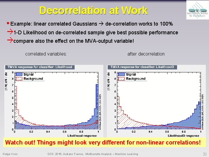
Decorrelation at Work § Example: linear correlated Gaussians de-correlation works to 100% 1 -D Likelihood on de-correlated sample give best possible performance compare also the effect on the MVA-output variable! correlated variables: after decorrelation Watch out! Things might look very different for non-linear correlations! Helge Voss SOS 2016, Autrans France, Multivariate Analysis – Machine Learning 31

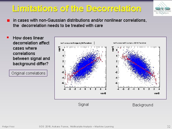
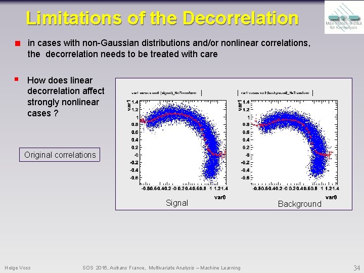
Limitations of the Decorrelation in cases with non-Gaussian distributions and/or nonlinear correlations, the decorrelation needs to be treated with care § How does linear decorrelation affect cases where correlations between signal and background differ? Original correlations Signal Helge Voss SOS 2016, Autrans France, Multivariate Analysis – Machine Learning Background 32

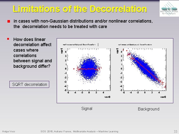
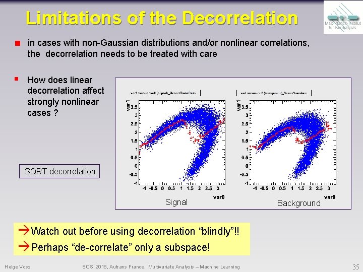
Limitations of the Decorrelation in cases with non-Gaussian distributions and/or nonlinear correlations, the decorrelation needs to be treated with care § How does linear decorrelation affect cases where correlations between signal and background differ? SQRT decorrelation Signal Helge Voss SOS 2016, Autrans France, Multivariate Analysis – Machine Learning Background 33

Limitations of the Decorrelation in cases with non-Gaussian distributions and/or nonlinear correlations, the decorrelation needs to be treated with care § How does linear decorrelation affect strongly nonlinear cases ? Original correlations Signal Helge Voss SOS 2016, Autrans France, Multivariate Analysis – Machine Learning Background 34

Limitations of the Decorrelation in cases with non-Gaussian distributions and/or nonlinear correlations, the decorrelation needs to be treated with care § How does linear decorrelation affect strongly nonlinear cases ? SQRT decorrelation Signal Background Watch out before using decorrelation “blindly”!! Perhaps “de-correlate” only a subspace! Helge Voss SOS 2016, Autrans France, Multivariate Analysis – Machine Learning 35

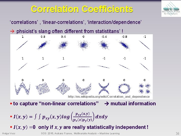
Correlation Coefficients ‘correlations’ , ‘linear-correlations’, ‘interaction/dependence’ phsicist’s slang often different from statistitans’ ! http: //en. wikipedia. org/wiki/Correlation_and_dependence § to capture “non-linear correlations” mutual information Helge Voss SOS 2016, Autrans France, Multivariate Analysis – Machine Learning 36

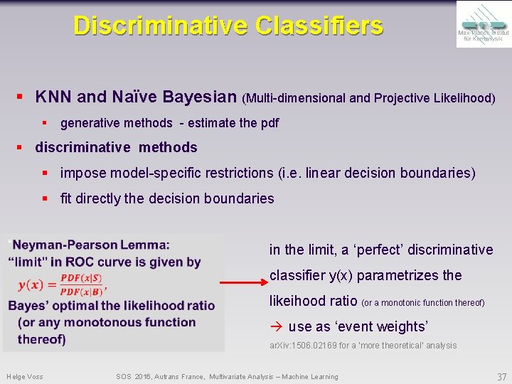
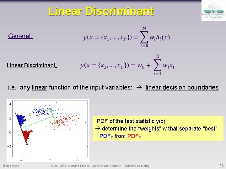
Discriminative Classifiers § KNN and Naïve Bayesian (Multi-dimensional and Projective Likelihood) § generative methods - estimate the pdf § discriminative methods § impose model-specific restrictions (i. e. linear decision boundaries) § fit directly the decision boundaries in the limit, a ‘perfect’ discriminative classifier y(x) parametrizes the likeihood ratio (or a monotonic function thereof) use as ‘event weights’ ar. Xiv: 1506. 02169 for a ‘more theoretical’ analysis Helge Voss SOS 2016, Autrans France, Multivariate Analysis – Machine Learning 37

Linear Discriminant General: Linear Discriminant: i. e. any linear function of the input variables: linear decision boundaries x 2 H 1 PDF of the test statistic y(x) determine the “weights” w that separate “best” PDFS from PDFB H 0 x 1 Helge Voss SOS 2016, Autrans France, Multivariate Analysis – Machine Learning 38

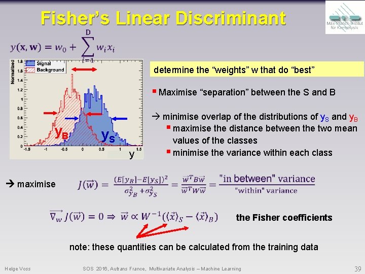
Fisher’s Linear Discriminant determine the “weights” w that do “best” § Maximise “separation” between the S and B y. S y maximise minimise overlap of the distributions of y. S and y. B § maximise the distance between the two mean values of the classes § minimise the variance within each class the Fisher coefficients note: these quantities can be calculated from the training data Helge Voss SOS 2016, Autrans France, Multivariate Analysis – Machine Learning 39

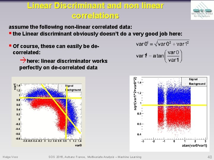
Linear Discriminant and non linear correlations assume the following non-linear correlated data: § the Linear discriminant obviously doesn’t do a very good job here: § Of course, these can easily be decorrelated: here: linear discriminator works perfectly on de-correlated data Helge Voss SOS 2016, Autrans France, Multivariate Analysis – Machine Learning 40

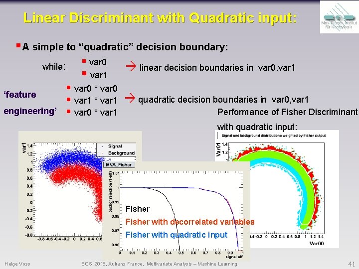
Linear Discriminant with Quadratic input: § A simple to “quadratic” decision boundary: while: ‘feature engineering’ § var 0 § var 1 linear decision boundaries in var 0, var 1 § var 0 * var 0 § var 1 * var 1 quadratic decision boundaries in var 0, var 1 Discriminant: Performance of Fisher Discriminant § var 0 * var 1 with quadratic input: Fisher with decorrelated variables Fisher with quadratic input Helge Voss SOS 2016, Autrans France, Multivariate Analysis – Machine Learning 41

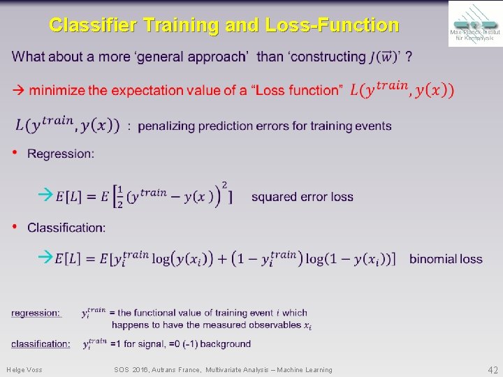
Classifier Training and Loss-Function Helge Voss SOS 2016, Autrans France, Multivariate Analysis – Machine Learning 42

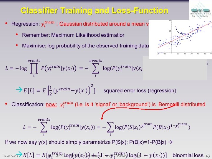
Classifier Training and Loss-Function Helge Voss SOS 2016, Autrans France, Multivariate Analysis – Machine Learning 43

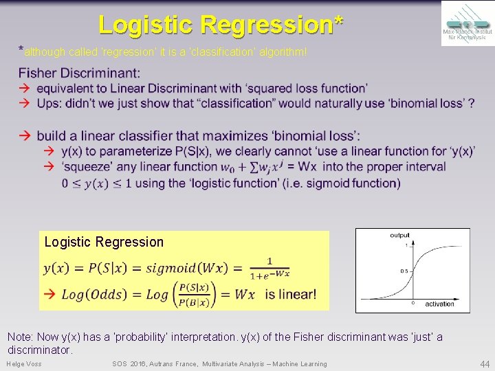
Logistic Regression* *although called ‘regression’ it is a ‘classification’ algorithm! Logistic Regression Note: Now y(x) has a ‘probability’ interpretation. y(x) of the Fisher discriminant was ‘just’ a discriminator. Helge Voss SOS 2016, Autrans France, Multivariate Analysis – Machine Learning 44

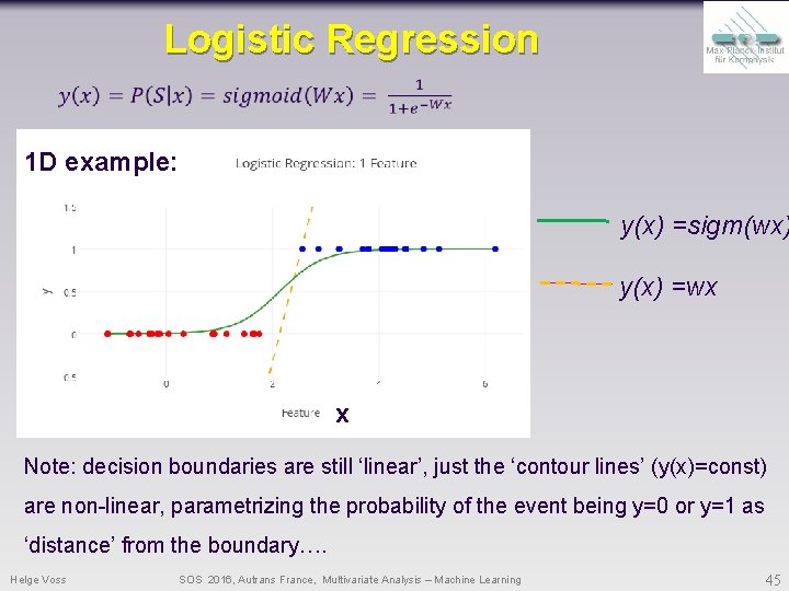
Logistic Regression 1 D example: y(x) =sigm(wx) y(x) =wx x Note: decision boundaries are still ‘linear’, just the ‘contour lines’ (y(x)=const) are non-linear, parametrizing the probability of the event being y=0 or y=1 as ‘distance’ from the boundary…. Helge Voss SOS 2016, Autrans France, Multivariate Analysis – Machine Learning 45

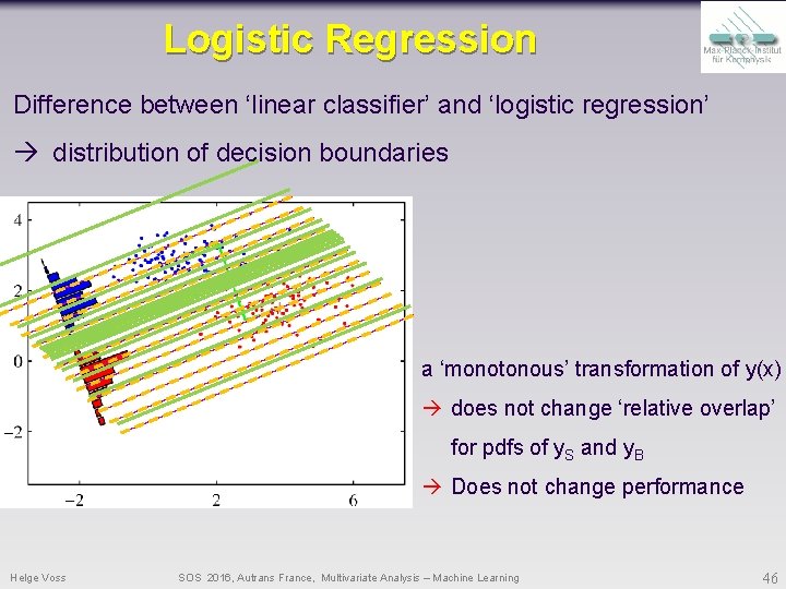
Logistic Regression Difference between ‘linear classifier’ and ‘logistic regression’ distribution of decision boundaries a ‘monotonous’ transformation of y(x) does not change ‘relative overlap’ for pdfs of y. S and y. B Does not change performance Helge Voss SOS 2016, Autrans France, Multivariate Analysis – Machine Learning 46

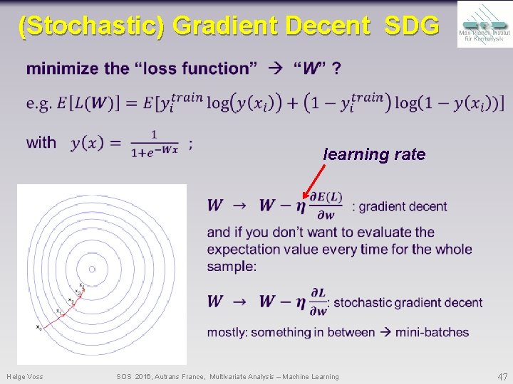
(Stochastic) Gradient Decent SDG learning rate Helge Voss SOS 2016, Autrans France, Multivariate Analysis – Machine Learning 47

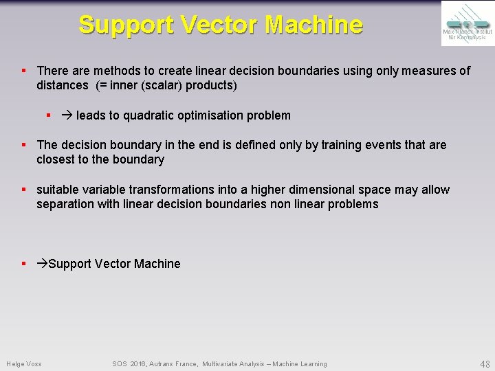
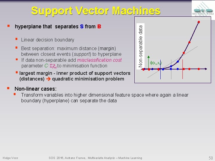
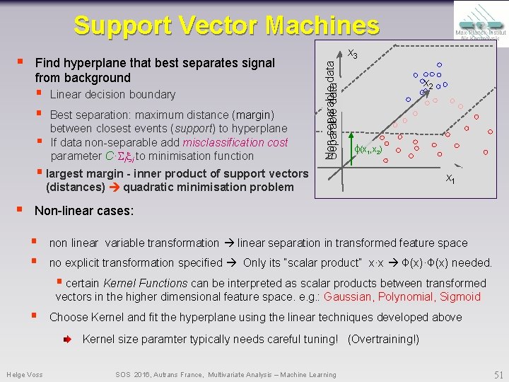
Support Vector Machine § There are methods to create linear decision boundaries using only measures of distances (= inner (scalar) products) § leads to quadratic optimisation problem § The decision boundary in the end is defined only by training events that are closest to the boundary § suitable variable transformations into a higher dimensional space may allow separation with linear decision boundaries non linear problems § Support Vector Machine Helge Voss SOS 2016, Autrans France, Multivariate Analysis – Machine Learning 48

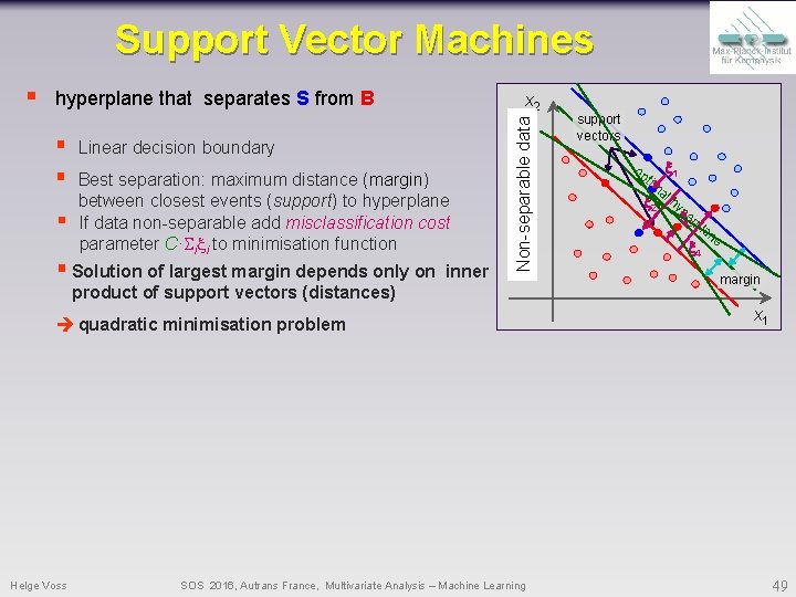
Support Vector Machines hyperplane that separates S from B § § § x 2 Linear decision boundary Best separation: maximum distance (margin) between closest events (support) to hyperplane If data non-separable add misclassification cost parameter C· i i to minimisation function § Solution of largest margin depends only on inner Separable data Non-separable § product of support vectors (distances) quadratic minimisation problem Helge Voss SOS 2016, Autrans France, Multivariate Analysis – Machine Learning support vectors op tim 1 a 2 l hyp e 3 rp la 4 ne margin x 1 49

§ hyperplane that separates S from B § § § Linear decision boundary Best separation: maximum distance (margin) between closest events (support) to hyperplane If data non-separable add misclassification cost parameter C· i i to minimisation function Separable data Non-separable Support Vector Machines (x 1, x 2) § largest margin - inner product of support vectors (distances) quadratic minimisation problem § Non-linear cases: § Helge Voss Transform variables into higher dimensional feature space where again a linear boundary (hyperplane) can separate the data SOS 2016, Autrans France, Multivariate Analysis – Machine Learning 50

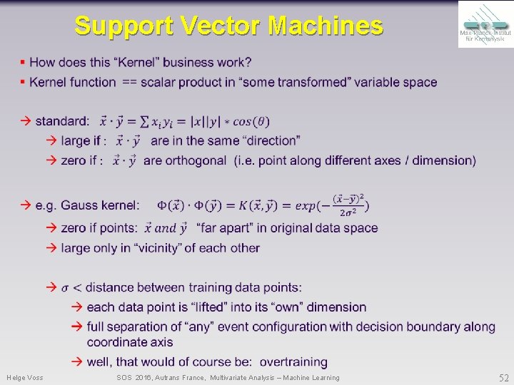
Support Vector Machines Find hyperplane that best separates signal from background § § § Linear decision boundary Best separation: maximum distance (margin) between closest events (support) to hyperplane If data non-separable add misclassification cost parameter C· i i to minimisation function Non-separable Separable data § x 3 xx 22 (x 1, x 2) § largest margin - inner product of support vectors (distances) quadratic minimisation problem § xx 11 x 1 Non-linear cases: § § non linear variable transformation linear separation in transformed feature space no explicit transformation specified Only its “scalar product” x·x Ф(x)·Ф(x) needed. § certain Kernel Functions can be interpreted as scalar products between transformed vectors in the higher dimensional feature space. e. g. : Gaussian, Polynomial, Sigmoid § Choose Kernel and fit the hyperplane using the linear techniques developed above Kernel size paramter typically needs careful tuning! (Overtraining!) Helge Voss SOS 2016, Autrans France, Multivariate Analysis – Machine Learning 51

Support Vector Machines Helge Voss SOS 2016, Autrans France, Multivariate Analysis – Machine Learning 52

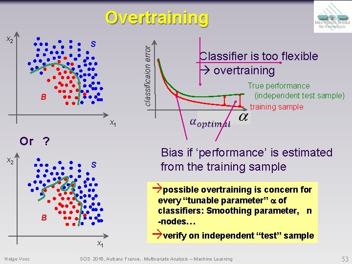
Overtraining x 2 classificaion error S B x 1 Or ? x 2 Classifier is too flexible overtraining True performance (independent test sample) training sample training cycles a Bias if ‘performance’ is estimated from the training sample S possible overtraining is concern for every “tunable parameter” a of classifiers: Smoothing parameter, n -nodes… B x 1 Helge Voss verify on independent “test” sample SOS 2016, Autrans France, Multivariate Analysis – Machine Learning 53

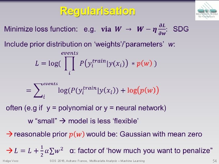
Regularisation Helge Voss SOS 2016, Autrans France, Multivariate Analysis – Machine Learning 54

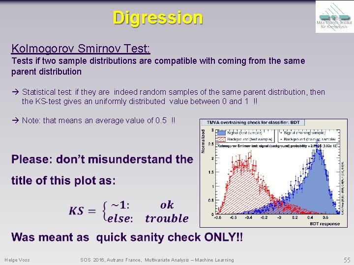
Digression Kolmogorov Smirnov Test: Tests if two sample distributions are compatible with coming from the same parent distribution Statistical test: if they are indeed random samples of the same parent distribution, then the KS-test gives an uniformly distributed value between 0 and 1 !! Note: that means an average value of 0. 5 !! Helge Voss SOS 2016, Autrans France, Multivariate Analysis – Machine Learning 55

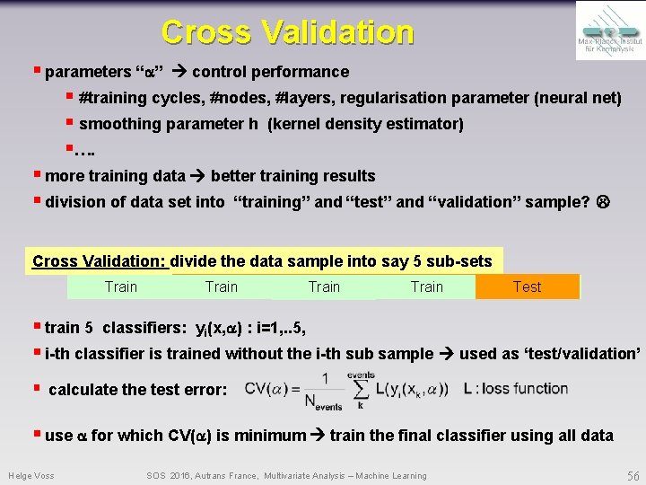
Cross Validation § parameters “a” control performance § #training cycles, #nodes, #layers, regularisation parameter (neural net) § smoothing parameter h (kernel density estimator) §…. § more training data better training results § division of data set into “training” and “test” and “validation” sample? Cross Validation: divide the data sample into say 5 sub-sets Test Train Test Train Train § train 5 classifiers: yi(x, a) : i=1, . . 5, § i-th classifier is trained without the i-th sub sample used as ‘test/validation’ § calculate the test error: § use a for which CV(a) is minimum train the final classifier using all data Helge Voss SOS 2016, Autrans France, Multivariate Analysis – Machine Learning 56

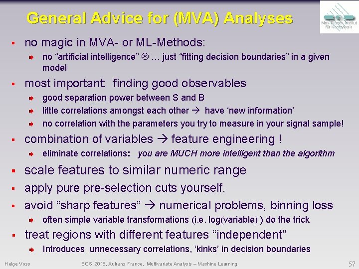
General Advice for (MVA) Analyses § no magic in MVA- or ML-Methods: no “artificial intelligence” … just “fitting decision boundaries” in a given model § most important: finding good observables good separation power between S and B little correlations amongst each other have ‘new information’ no correlation with the parameters you try to measure in your signal sample! § combination of variables feature engineering ! eliminate correlations: you are MUCH more intelligent than the algorithm § scale features to similar numeric range § apply pure pre-selection cuts yourself. avoid “sharp features” numerical problems, binning loss § often simple variable transformations (i. e. log(variable) ) do the trick § treat regions with different features “independent” Introduces unnecessary correlations, ‘kinks’ in decision boundaries Helge Voss SOS 2016, Autrans France, Multivariate Analysis – Machine Learning 57

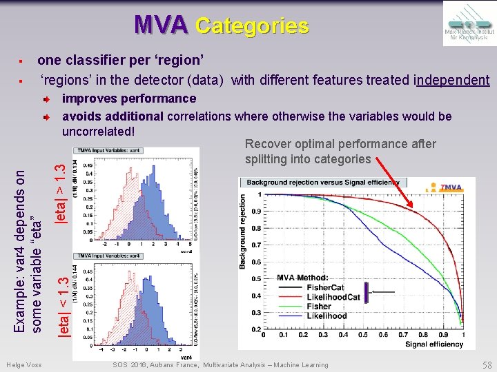
MVA Categories § § one classifier per ‘region’ ‘regions’ in the detector (data) with different features treated independent Helge Voss |eta| > 1. 3 |eta| < 1. 3 Example: var 4 depends on some variable “eta” improves performance avoids additional correlations where otherwise the variables would be uncorrelated! Recover optimal performance after splitting into categories SOS 2016, Autrans France, Multivariate Analysis – Machine Learning 58

About Systematic Errors Helge Voss SOS 2016, Autrans France, Multivariate Analysis – Machine Learning 59

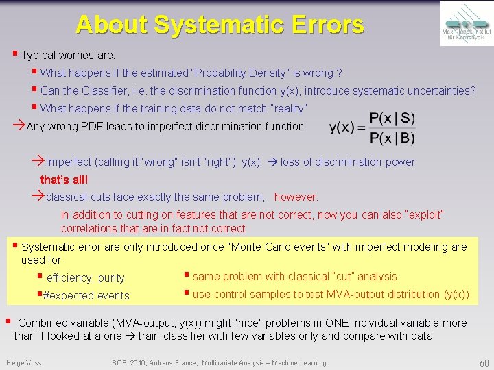
About Systematic Errors § Typical worries are: § What happens if the estimated “Probability Density” is wrong ? § Can the Classifier, i. e. the discrimination function y(x), introduce systematic uncertainties? § What happens if the training data do not match “reality” Any wrong PDF leads to imperfect discrimination function Imperfect (calling it “wrong” isn’t “right”) y(x) loss of discrimination power that’s all! classical cuts face exactly the same problem, however: in addition to cutting on features that are not correct, now you can also “exploit” correlations that are in fact not correct § Systematic error are only introduced once “Monte Carlo events” with imperfect modeling are used for § efficiency; purity §#expected events § § same problem with classical “cut” analysis § use control samples to test MVA-output distribution (y(x)) Combined variable (MVA-output, y(x)) might “hide” problems in ONE individual variable more than if looked at alone train classifier with few variables only and compare with data Helge Voss SOS 2016, Autrans France, Multivariate Analysis – Machine Learning 60

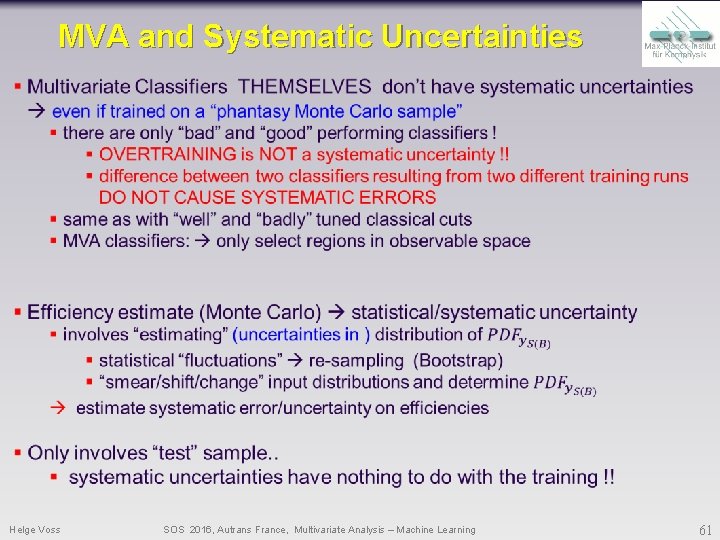
MVA and Systematic Uncertainties Helge Voss SOS 2016, Autrans France, Multivariate Analysis – Machine Learning 61

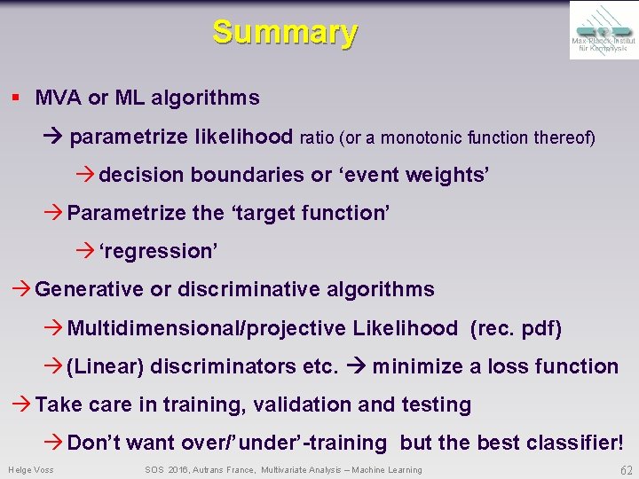
Summary § MVA or ML algorithms parametrize likelihood ratio (or a monotonic function thereof) decision boundaries or ‘event weights’ Parametrize the ‘target function’ ‘regression’ Generative or discriminative algorithms Multidimensional/projective Likelihood (rec. pdf) (Linear) discriminators etc. minimize a loss function Take care in training, validation and testing Don’t want over/’under’-training but the best classifier! Helge Voss SOS 2016, Autrans France, Multivariate Analysis – Machine Learning 62

Backup Helge Voss SOS 2016, Autrans France, Multivariate Analysis – Machine Learning 63

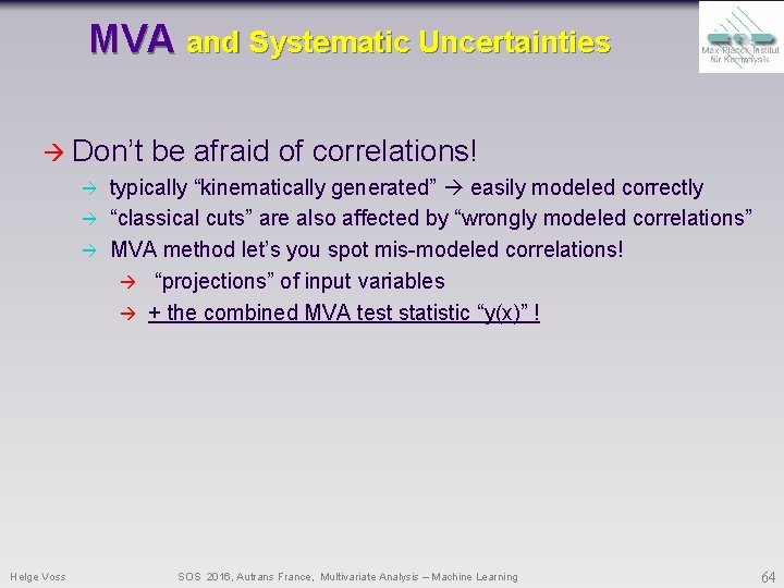
MVA and Systematic Uncertainties Don’t Helge Voss be afraid of correlations! typically “kinematically generated” easily modeled correctly “classical cuts” are also affected by “wrongly modeled correlations” MVA method let’s you spot mis-modeled correlations! “projections” of input variables + the combined MVA test statistic “y(x)” ! SOS 2016, Autrans France, Multivariate Analysis – Machine Learning 64

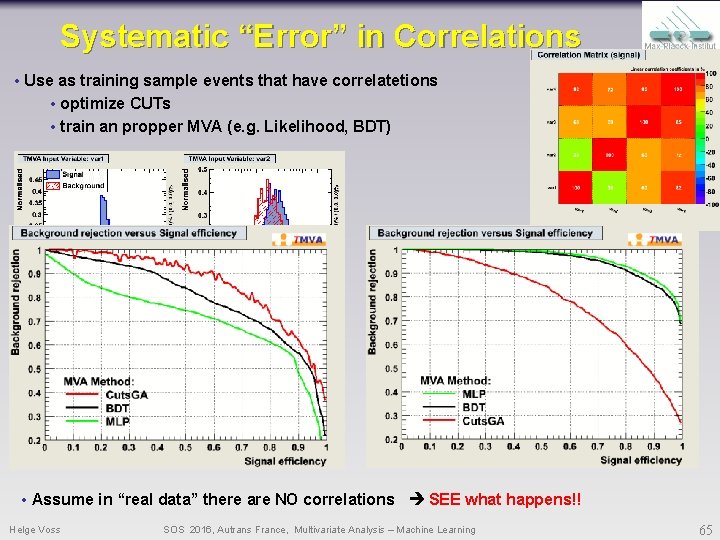
Systematic “Error” in Correlations • Use as training sample events that have correlatetions • optimize CUTs • train an propper MVA (e. g. Likelihood, BDT) • Assume in “real data” there are NO correlations SEE what happens!! Helge Voss SOS 2016, Autrans France, Multivariate Analysis – Machine Learning 65

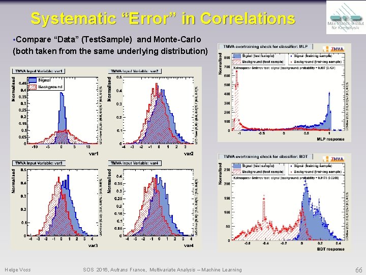
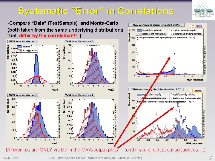
Systematic “Error” in Correlations • Compare “Data” (Test. Sample) and Monte-Carlo (both taken from the same underlying distribution) Helge Voss SOS 2016, Autrans France, Multivariate Analysis – Machine Learning 66

Systematic “Error” in Correlations • Compare “Data” (Test. Sample) and Monte-Carlo (both taken from the same underlying distributions that differ by the correlation!!! ) Differences are ONLY visible in the MVA-output plots Helge Voss (and if you’d look at cut sequences…. ) SOS 2016, Autrans France, Multivariate Analysis – Machine Learning 67

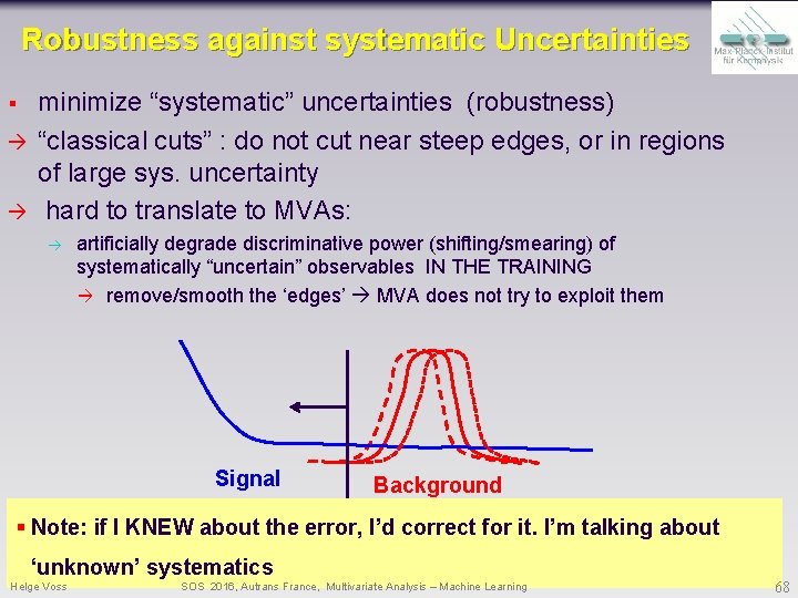
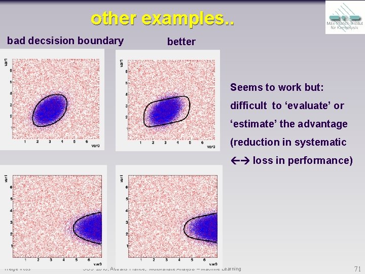
Robustness against systematic Uncertainties § minimize “systematic” uncertainties (robustness) “classical cuts” : do not cut near steep edges, or in regions of large sys. uncertainty hard to translate to MVAs: artificially degrade discriminative power (shifting/smearing) of systematically “uncertain” observables IN THE TRAINING remove/smooth the ‘edges’ MVA does not try to exploit them Signal Background § Note: if I KNEW about the error, I’d correct for it. I’m talking about ‘unknown’ systematics Helge Voss SOS 2016, Autrans France, Multivariate Analysis – Machine Learning 68

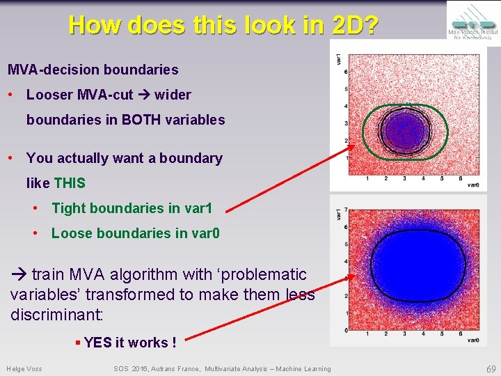
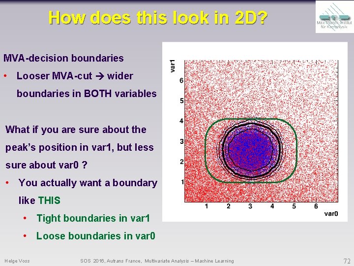
How does this look in 2 D? MVA-decision boundaries • Looser MVA-cut wider boundaries in BOTH variables • You actually want a boundary like THIS • Tight boundaries in var 1 • Loose boundaries in var 0 train MVA algorithm with ‘problematic variables’ transformed to make them less discriminant: § YES it works ! Helge Voss SOS 2016, Autrans France, Multivariate Analysis – Machine Learning 69

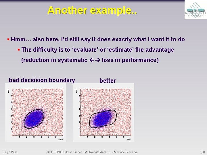
Another example. . § Hmm… also here, I’d still say it does exactly what I want it to do § The difficulty is to ‘evaluate’ or ‘estimate’ the advantage (reduction in systematic loss in performance) bad decsision boundary Helge Voss better SOS 2016, Autrans France, Multivariate Analysis – Machine Learning 70

other examples. . bad decsision boundary better Seems to work but: difficult to ‘evaluate’ or ‘estimate’ the advantage (reduction in systematic loss in performance) Helge Voss SOS 2016, Autrans France, Multivariate Analysis – Machine Learning 71

How does this look in 2 D? MVA-decision boundaries • Looser MVA-cut wider boundaries in BOTH variables What if you are sure about the peak’s position in var 1, but less sure about var 0 ? • You actually want a boundary like THIS • Tight boundaries in var 1 • Loose boundaries in var 0 Helge Voss SOS 2016, Autrans France, Multivariate Analysis – Machine Learning 72

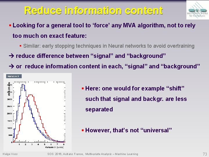
Reduce information content § Looking for a general tool to ‘force’ any MVA algorithm, not to rely too much on exact feature: § Similar: early stopping techniques in Neural networks to avoid overtraining reduce difference between “signal” and “background” or reduce information content in each, “signal” and “background” § Here: one would for example “shift” such that signal and backgr. are less separated § However, that’s not “universal” Helge Voss SOS 2016, Autrans France, Multivariate Analysis – Machine Learning 73

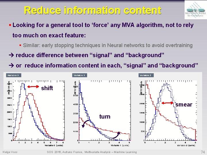
Reduce information content § Looking for a general tool to ‘force’ any MVA algorithm, not to rely too much on exact feature: § Similar: early stopping techniques in Neural networks to avoid overtraining reduce difference between “signal” and “background” or reduce information content in each, “signal” and “background” shift smear turn Helge Voss SOS 2016, Autrans France, Multivariate Analysis – Machine Learning 74

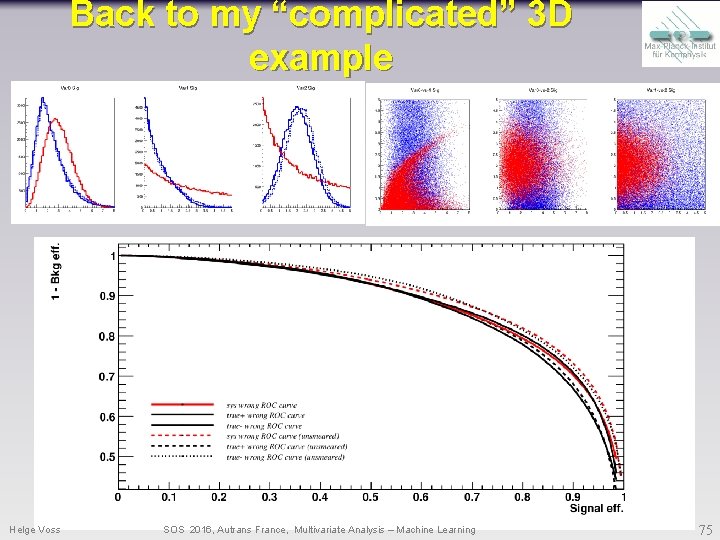
Back to my “complicated” 3 D example Helge Voss SOS 2016, Autrans France, Multivariate Analysis – Machine Learning 75

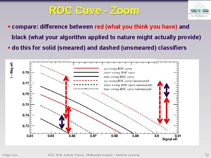
ROC Cuve - Zoom § compare: difference between red (what you think you have) and black (what your algorithm applied to nature might actually provide) § do this for solid (smeared) and dashed (unsmeared) classifiers Helge Voss SOS 2016, Autrans France, Multivariate Analysis – Machine Learning 76

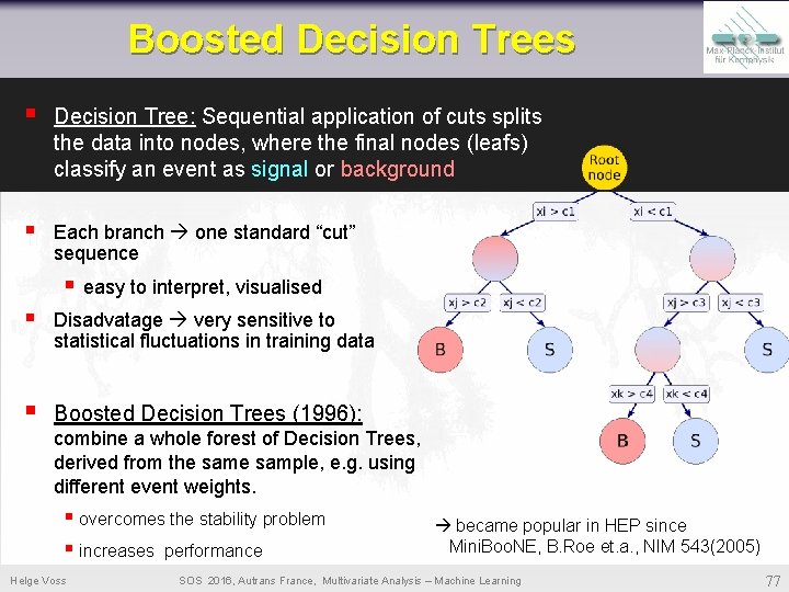
Boosted Decision Trees § Decision Tree: Sequential application of cuts splits the data into nodes, where the final nodes (leafs) classify an event as signal or background § Each branch one standard “cut” sequence § easy to interpret, visualised § Disadvatage very sensitive to statistical fluctuations in training data § Boosted Decision Trees (1996): combine a whole forest of Decision Trees, derived from the sample, e. g. using different event weights. § overcomes the stability problem § increases performance Helge Voss became popular in HEP since Mini. Boo. NE, B. Roe et. a. , NIM 543(2005) SOS 2016, Autrans France, Multivariate Analysis – Machine Learning 77

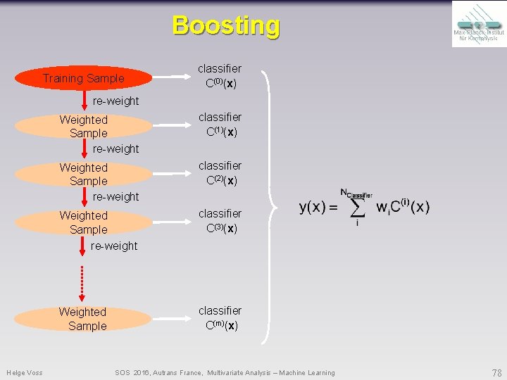
Boosting Training Sample classifier C(0)(x) re-weight Helge Voss Weighted Sample re-weight classifier C(1)(x) Weighted Sample re-weight classifier C(2)(x) Weighted Sample re-weight classifier C(3)(x) Weighted Sample classifier C(m)(x) SOS 2016, Autrans France, Multivariate Analysis – Machine Learning 78

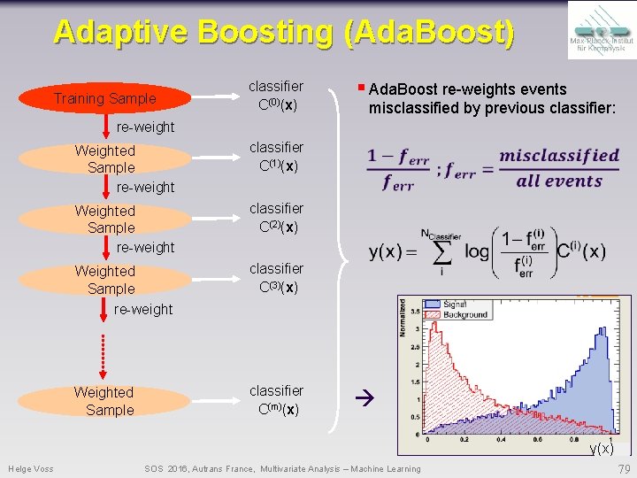
Adaptive Boosting (Ada. Boost) Training Sample § Ada. Boost re-weights events classifier C(0)(x) re-weight Weighted Sample re-weight classifier C(1)(x) Weighted Sample re-weight classifier C(2)(x) Weighted Sample re-weight classifier C(3)(x) Weighted Sample classifier C(m)(x) misclassified by previous classifier: y(x) Helge Voss SOS 2016, Autrans France, Multivariate Analysis – Machine Learning 79

Boosted Decision Trees § Are very popular in HEP § Robust and easy to train, § get good results § But: when we adopted BDTs, § In 2006 ANNs just started their big breakthrough in the ML community with remarkable advances in DEEP Learning ! Let’s move on to Neural Networks Helge Voss SOS 2016, Autrans France, Multivariate Analysis – Machine Learning 80

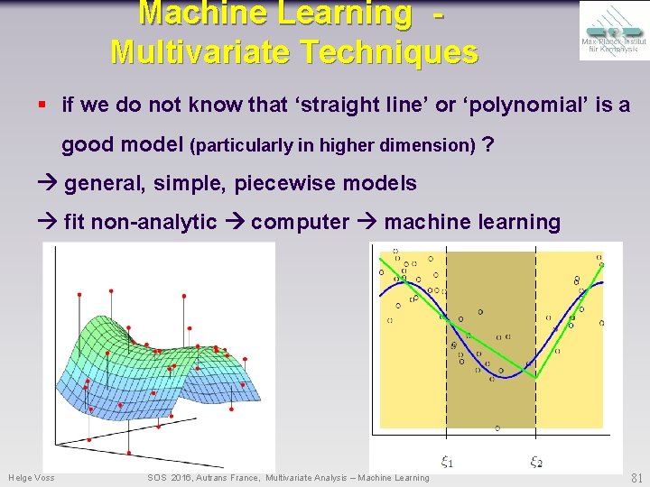
Machine Learning Multivariate Techniques § if we do not know that ‘straight line’ or ‘polynomial’ is a good model (particularly in higher dimension) ? general, simple, piecewise models fit non-analytic computer machine learning Helge Voss SOS 2016, Autrans France, Multivariate Analysis – Machine Learning 81

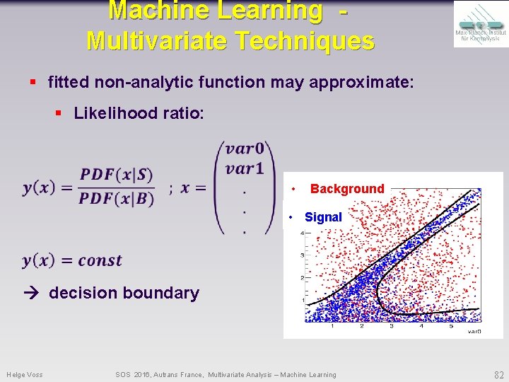
Machine Learning Multivariate Techniques § fitted non-analytic function may approximate: § Likelihood ratio: • Background • Signal decision boundary Helge Voss SOS 2016, Autrans France, Multivariate Analysis – Machine Learning 82

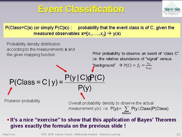
Event Classification P(Class=C|x) (or simply P(C|x)) : probability that the event class is of C, given the measured observables x={x 1, …. , x. D} y(x) Probability density distribution according to the measurements x and the given mapping function Posterior probability Overall probability density to observe the actual measurement y(x). i. e. § It’s a nice “exercise” to show that this application of Bayes’ Theorem gives exactly the formula on the previous slide ! Helge Voss SOS 2016, Autrans France, Multivariate Analysis – Machine Learning 83

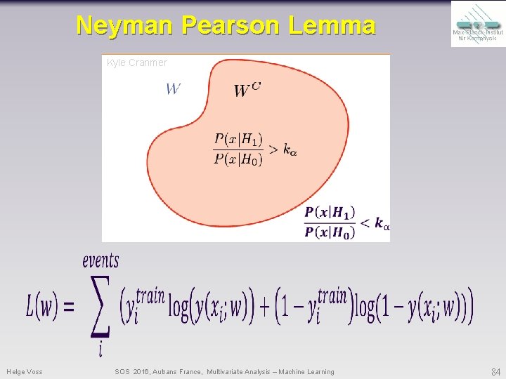
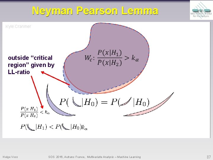
Neyman Pearson Lemma Kyle Cranmer Helge Voss SOS 2016, Autrans France, Multivariate Analysis – Machine Learning 84

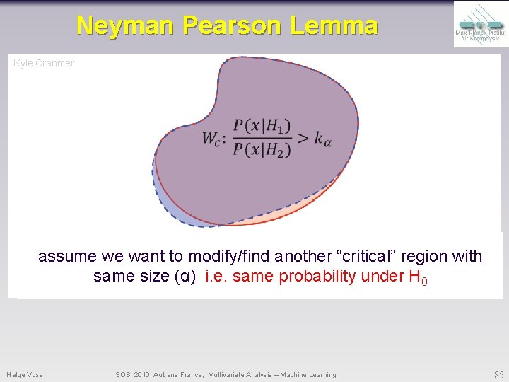
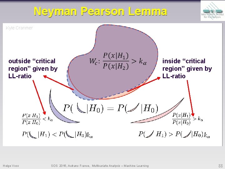
Neyman Pearson Lemma Kyle Cranmer assume we want to modify/find another “critical” region with same size (α) i. e. same probability under H 0 Helge Voss SOS 2016, Autrans France, Multivariate Analysis – Machine Learning 85

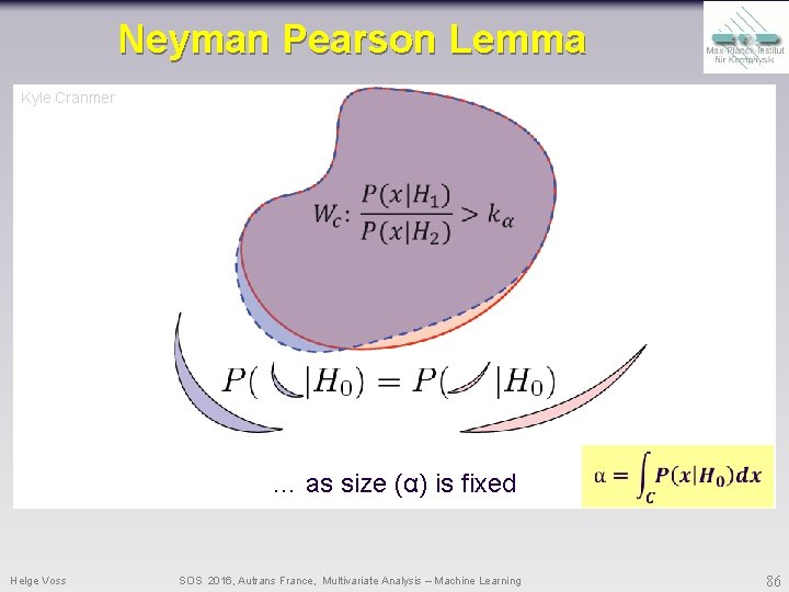
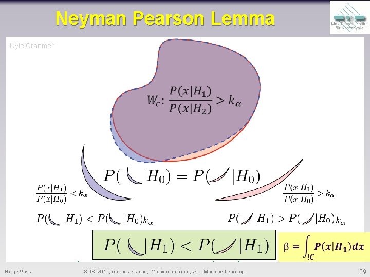
Neyman Pearson Lemma Kyle Cranmer … as size (α) is fixed Helge Voss SOS 2016, Autrans France, Multivariate Analysis – Machine Learning 86

Neyman Pearson Lemma Kyle Cranmer outside “critical region” given by LL-ratio Helge Voss SOS 2016, Autrans France, Multivariate Analysis – Machine Learning 87

Neyman Pearson Lemma Kyle Cranmer outside “critical region” given by LL-ratio Helge Voss SOS 2016, Autrans France, Multivariate Analysis – Machine Learning inside “critical region” given by LL-ratio 88

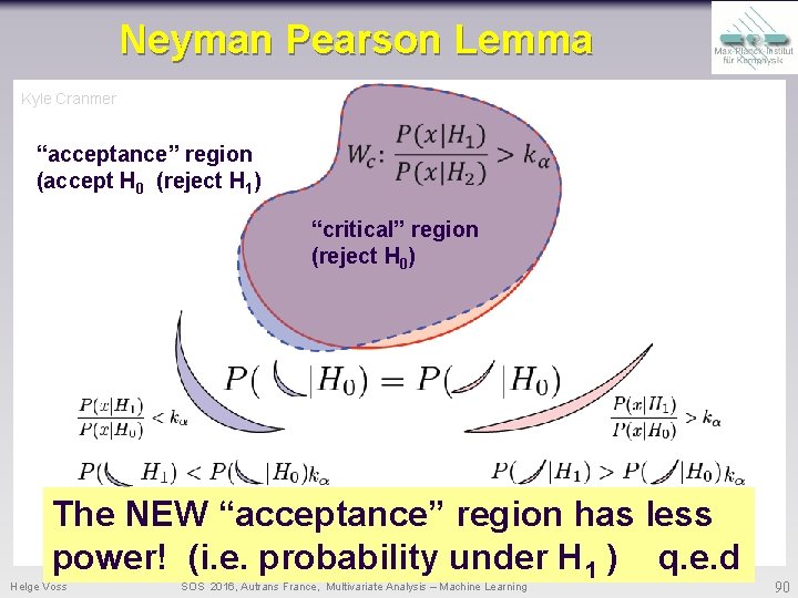
Neyman Pearson Lemma Kyle Cranmer Helge Voss SOS 2016, Autrans France, Multivariate Analysis – Machine Learning 89

Neyman Pearson Lemma Kyle Cranmer “acceptance” region (accept H 0 (reject H 1) “critical” region (reject H 0) The NEW “acceptance” region has less power! (i. e. probability under H 1 ) q. e. d Helge Voss SOS 2016, Autrans France, Multivariate Analysis – Machine Learning 90