Lecture Slides for INTRODUCTION TO Machine Learning ETHEM

Lecture Slides for INTRODUCTION TO Machine Learning ETHEM ALPAYDIN © The MIT Press, 2010 alpaydin@boun. edu. tr http: //www. cmpe. boun. edu. tr/~ethem/i 2 ml 2 e

CHAPTER 2: Supervised Learning

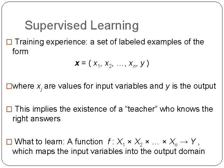
Supervised Learning � Training experience: a set of labeled examples of the form x = ( x 1, x 2, …, xn, y ) �where xj are values for input variables and y is the output � This implies the existence of a “teacher” who knows the right answers � What to learn: A function f : X 1 × X 2 × … × Xn → Y , 3 which maps the input variables into the output domain

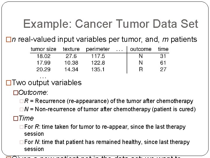
Example: Cancer Tumor Data Set �n real-valued input variables per tumor, and, m patients �Two output variables �Outcome: �R = Recurrence (re-appearance) of the tumor after chemotherapy �N = Non-recurrence of tumor after chemotherapy (patient is cured) 4 �Time �For R: time taken for tumor to re-appear, since the last therapy session �For N: time that patient has remained healthy, since last therapy session

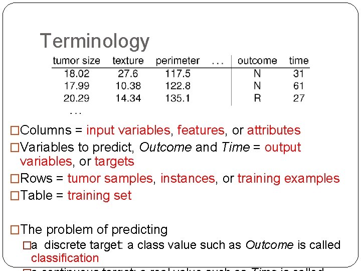
Terminology �Columns = input variables, features, or attributes �Variables to predict, Outcome and Time = output variables, or targets �Rows = tumor samples, instances, or training examples �Table = training set �The problem of predicting 5 �a discrete target: a class value such as Outcome is called classification

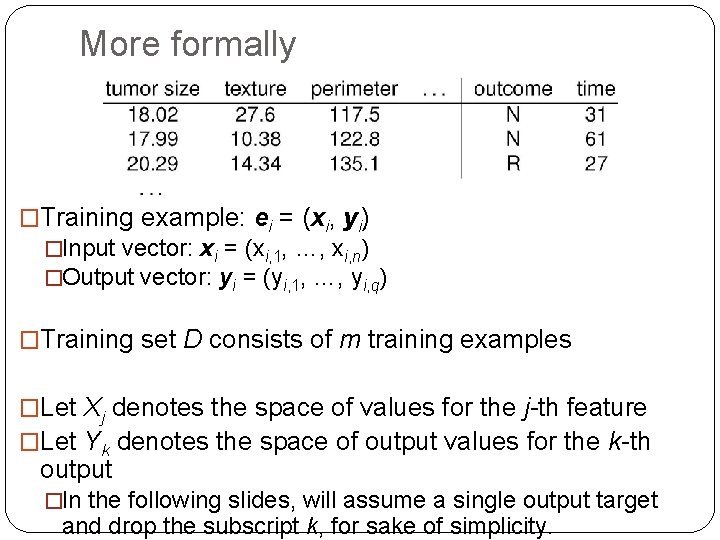
More formally �Training example: ei = (xi, yi) �Input vector: xi = (xi, 1, …, xi, n) �Output vector: yi = (yi, 1, …, yi, q) �Training set D consists of m training examples �Let Xj denotes the space of values for the j-th feature �Let Yk denotes the space of output values for the k-th output 6 �In the following slides, will assume a single output target and drop the subscript k, for sake of simplicity.

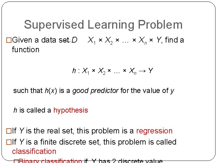
Supervised Learning Problem �Given a data set D function X 1 × X 2 × … × Xn × Y, find a h : X 1 × X 2 × … × Xn → Y such that h(x) is a good predictor for the value of y h is called a hypothesis �If Y is the real set, this problem is a regression �If Y is a finite discrete set, this problem is called 7 classification

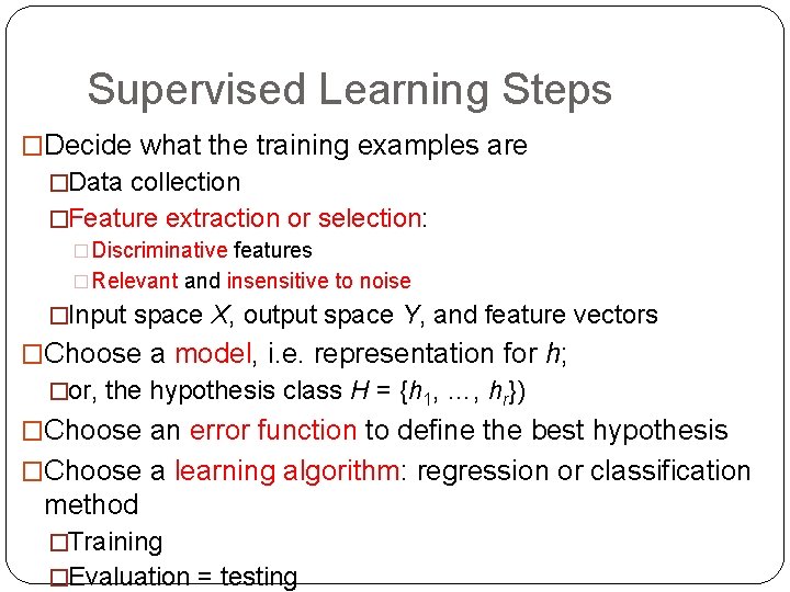
Supervised Learning Steps �Decide what the training examples are �Data collection �Feature extraction or selection: �Discriminative features �Relevant and insensitive to noise �Input space X, output space Y, and feature vectors �Choose a model, i. e. representation for h; �or, the hypothesis class H = {h 1, …, hr}) �Choose an error function to define the best hypothesis �Choose a learning algorithm: regression or classification method 8 �Training �Evaluation = testing

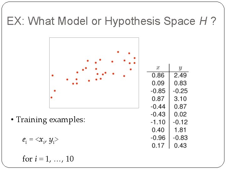
EX: What Model or Hypothesis Space H ? • Training examples: ei = <xi, yi> 9 for i = 1, …, 10

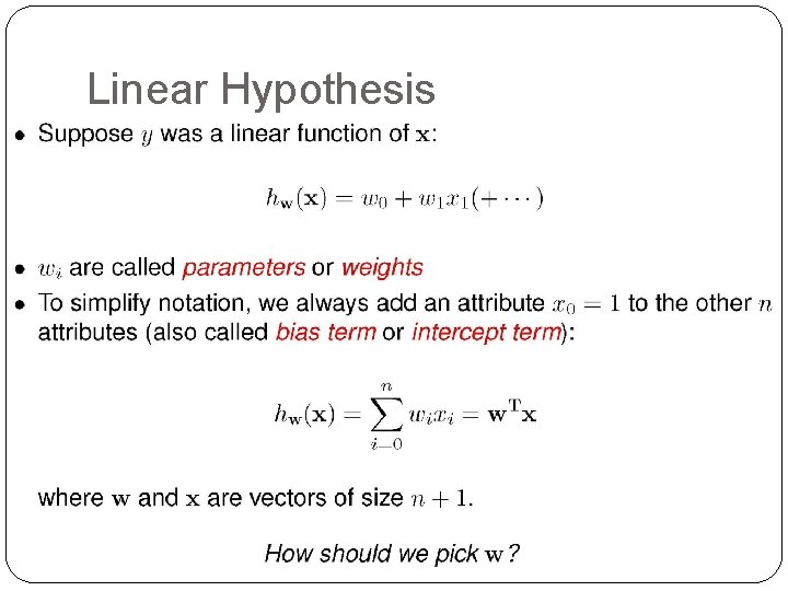
Linear Hypothesis 10

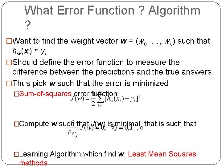
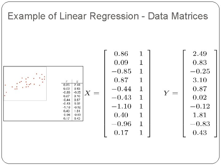
What Error Function ? Algorithm ? �Want to find the weight vector w = (w 0, …, wn) such that hw(xi) ≈ yi �Should define the error function to measure the difference between the predictions and the true answers �Thus pick w such that the error is minimized �Sum-of-squares error function: �Compute w such that J(w) is minimal, that is such that: 11 �Learning Algorithm which find w: Least Mean Squares methods

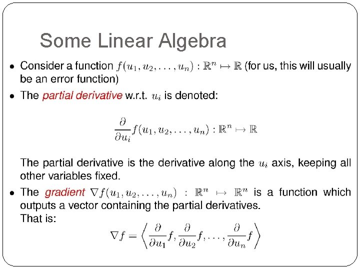
Some Linear Algebra 12

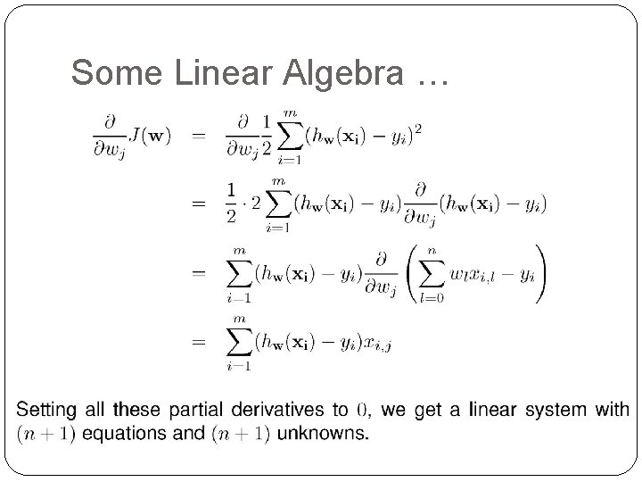
Some Linear Algebra … 13

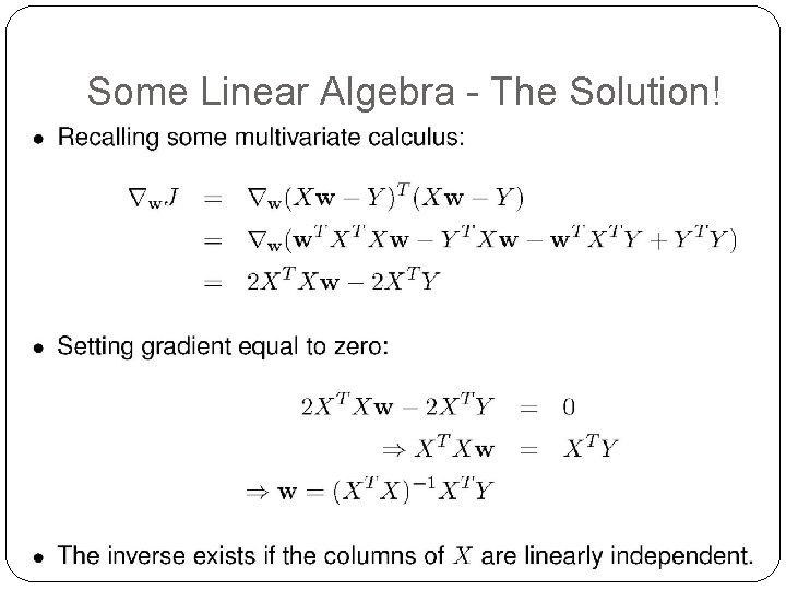
Some Linear Algebra - The Solution! 14

Example of Linear Regression - Data Matrices 15

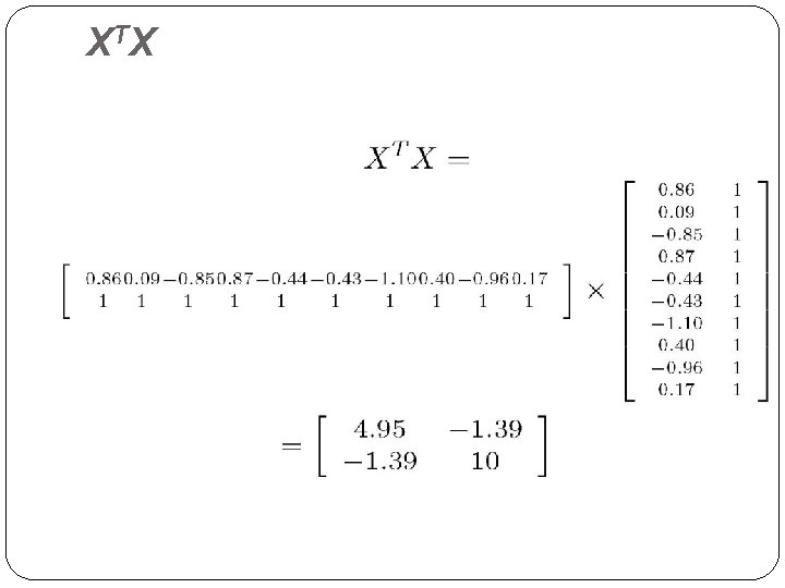
X TX 16

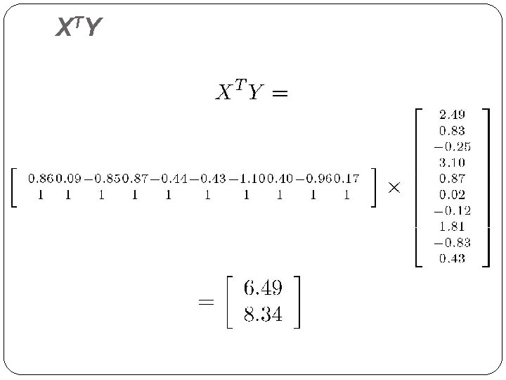
X TY 17

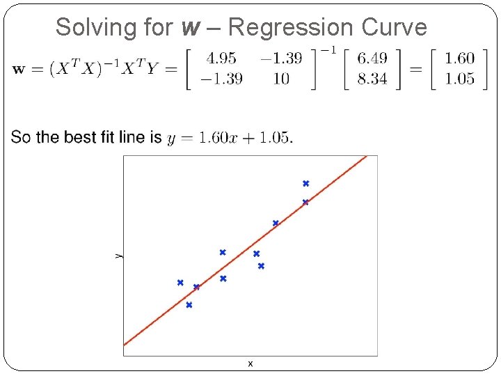
Solving for w – Regression Curve 18

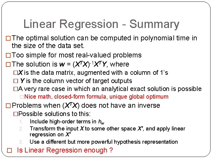
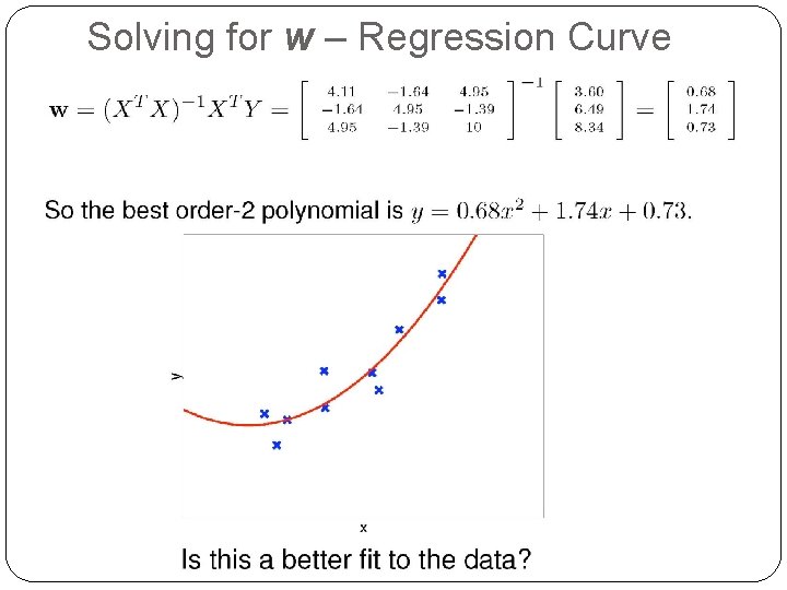
Linear Regression - Summary � The optimal solution can be computed in polynomial time in the size of the data set. � Too simple for most real-valued problems � The solution is w = (XTX)-1 XTY, where �X is the data matrix, augmented with a column of 1’s � Y is the column vector of target outputs �A very rare case in which an analytical exact solution is possible �Nice math, closed-formula, unique global optimum � Problems when (XTX) does not have an inverse �Possible solutions to this: 1. Include high-order terms in hw 2. Transform the input X to some other space X’, and apply linear regression on X’ 3. Use a different but more powerful hypothesis representation 19 � Is Linear Regression enough ?

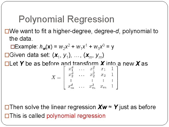
Polynomial Regression �We want to fit a higher-degree, degree-d, polynomial to the data. �Example: hw(x) = w 2 x 2 + w 1 x 1 + w 0 x 0 = y �Given data set: (x 1, y 1), …, (xm, ym) �Let Y be as before and transform X into a new X as �Then solve the linear regression Xw ≈ Y just as before � This is called polynomial regression 20

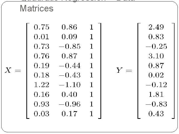
Quadratic Regression – Data Matrices 21

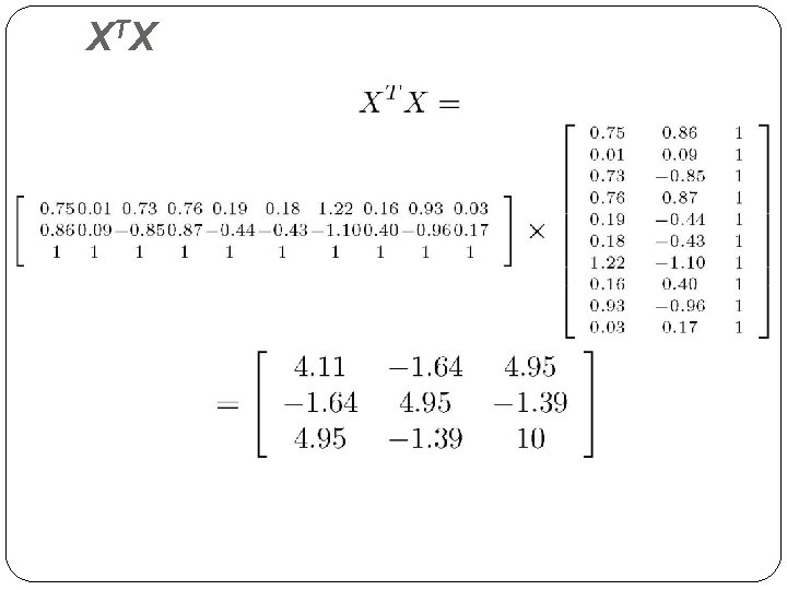
X TX 22

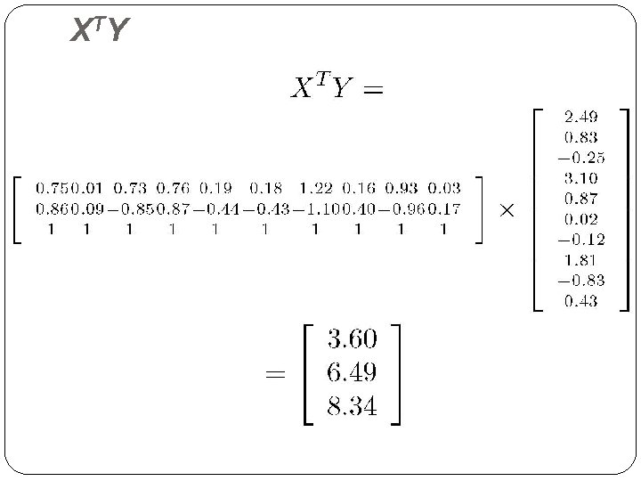
X TY 23

Solving for w – Regression Curve 24

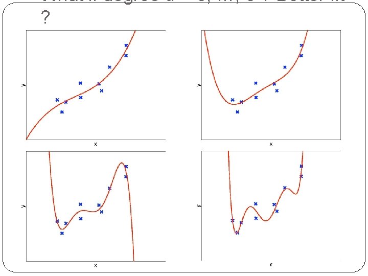
What if degree d = 3, …, 6 ? Better fit ? 25

What if degree d = 7, …, 9 ? Better fit ? 26

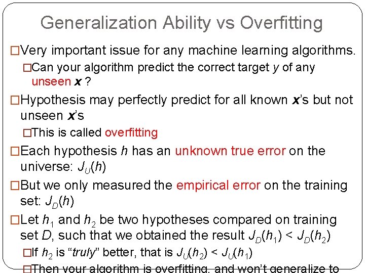
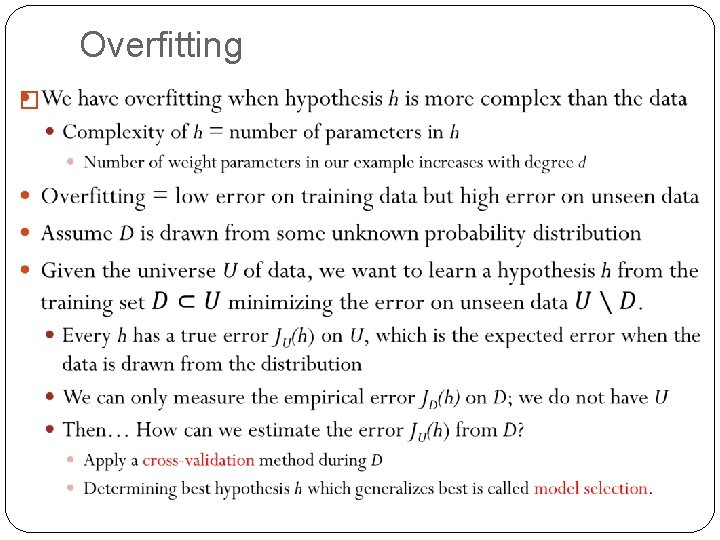
Generalization Ability vs Overfitting �Very important issue for any machine learning algorithms. �Can your algorithm predict the correct target y of any unseen x ? �Hypothesis may perfectly predict for all known x’s but not unseen x’s �This is called overfitting �Each hypothesis h has an unknown true error on the universe: JU(h) �But we only measured the empirical error on the training set: JD(h) �Let h 1 and h 2 be two hypotheses compared on training set D, such that we obtained the result JD(h 1) < JD(h 2) 27 �If h 2 is “truly” better, that is JU(h 2) < JU(h 1) �Then your algorithm is overfitting, and won’t generalize to

Overfitting � 28

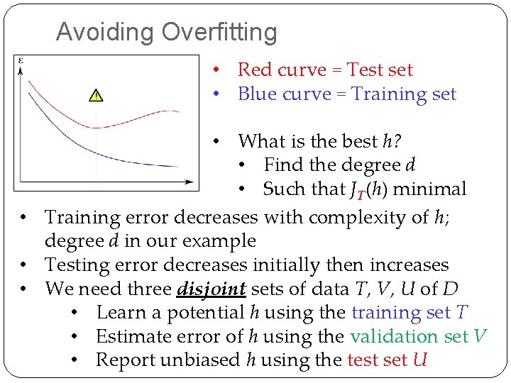
Avoiding Overfitting • Red curve = Test set • Blue curve = Training set • What is the best h? • Find the degree d • Such that JT(h) minimal • Training error decreases with complexity of h; degree d in our example • Testing error decreases initially then increases • We need three disjoint sets of data T, V, U of D • Learn a potential h using the training set T • Estimate error of h using the validation set V 29 • Report unbiased h using the test set U

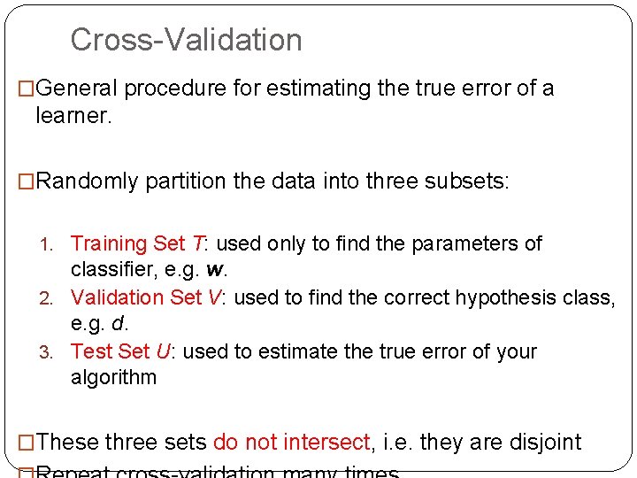
Cross-Validation �General procedure for estimating the true error of a learner. �Randomly partition the data into three subsets: 1. Training Set T: used only to find the parameters of classifier, e. g. w. 2. Validation Set V: used to find the correct hypothesis class, e. g. d. 3. Test Set U: used to estimate the true error of your algorithm � 30 These three sets do not intersect, i. e. they are disjoint

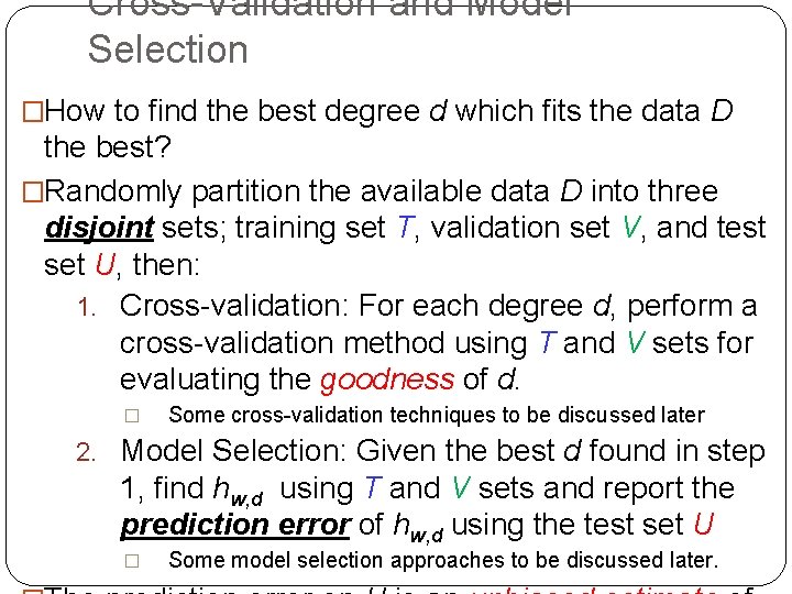
Cross-Validation and Model Selection �How to find the best degree d which fits the data D the best? �Randomly partition the available data D into three disjoint sets; training set T, validation set V, and test set U, then: 1. Cross-validation: For each degree d, perform a cross-validation method using T and V sets for evaluating the goodness of d. � Some cross-validation techniques to be discussed later 2. Model Selection: Given the best d found in step 1, find hw, d using T and V sets and report the prediction error of hw, d using the test set U 31 � Some model selection approaches to be discussed later.

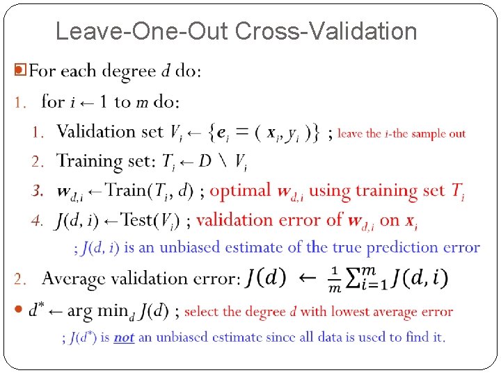
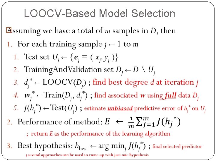
Leave-One-Out Cross-Validation � 32

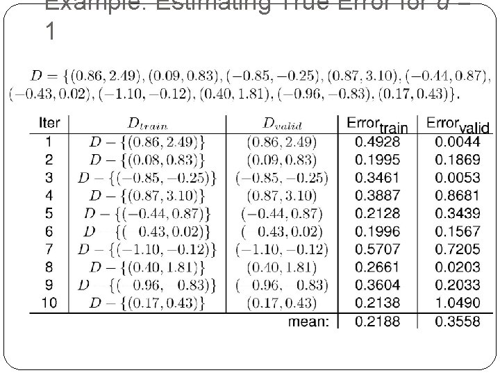
Example: Estimating True Error for d = 1 33

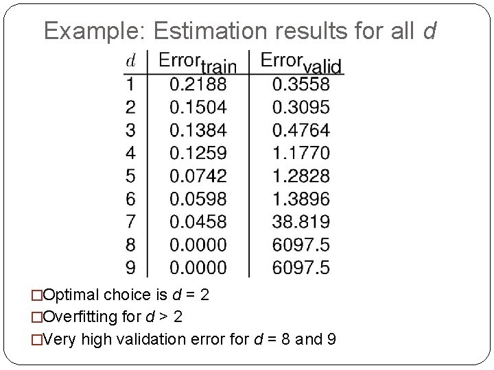
Example: Estimation results for all d �Optimal choice is d = 2 �Overfitting for d > 2 34 �Very high validation error for d = 8 and 9

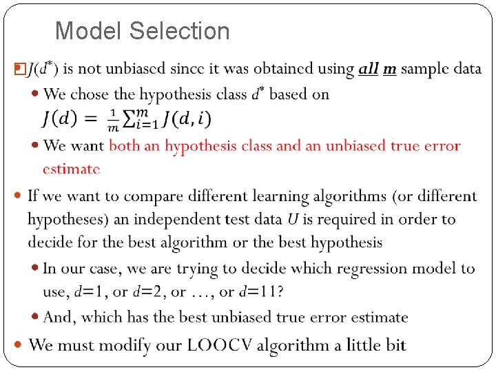
Model Selection � 35

LOOCV-Based Model Selection � 36

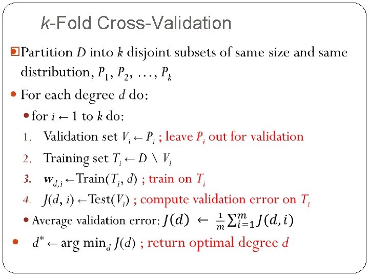
k-Fold Cross-Validation � 37

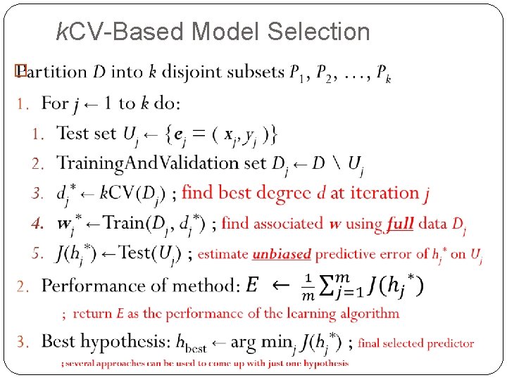
k. CV-Based Model Selection � 38

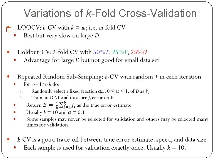
Variations of k-Fold Cross-Validation � 39

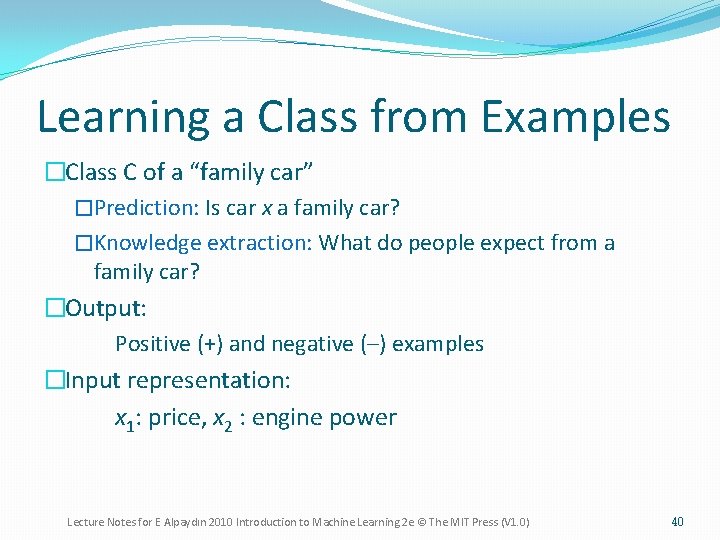
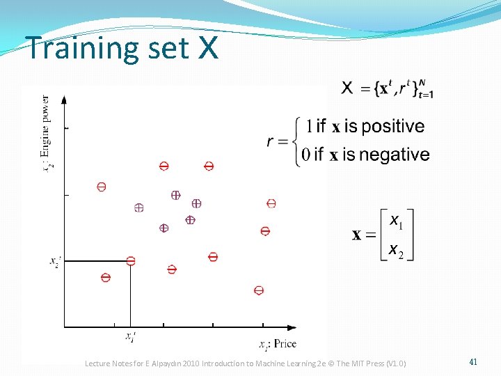
Learning a Class from Examples �Class C of a “family car” �Prediction: Is car x a family car? �Knowledge extraction: What do people expect from a family car? �Output: Positive (+) and negative (–) examples �Input representation: x 1: price, x 2 : engine power Lecture Notes for E Alpaydın 2010 Introduction to Machine Learning 2 e © The MIT Press (V 1. 0) 40

Training set X Lecture Notes for E Alpaydın 2010 Introduction to Machine Learning 2 e © The MIT Press (V 1. 0) 41

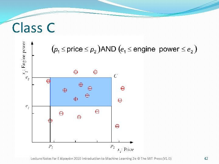
Class C Lecture Notes for E Alpaydın 2010 Introduction to Machine Learning 2 e © The MIT Press (V 1. 0) 42

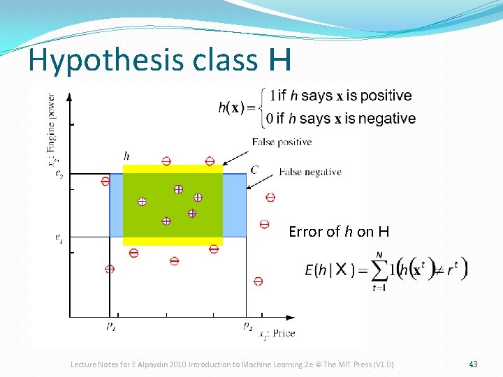
Hypothesis class H Error of h on H Lecture Notes for E Alpaydın 2010 Introduction to Machine Learning 2 e © The MIT Press (V 1. 0) 43

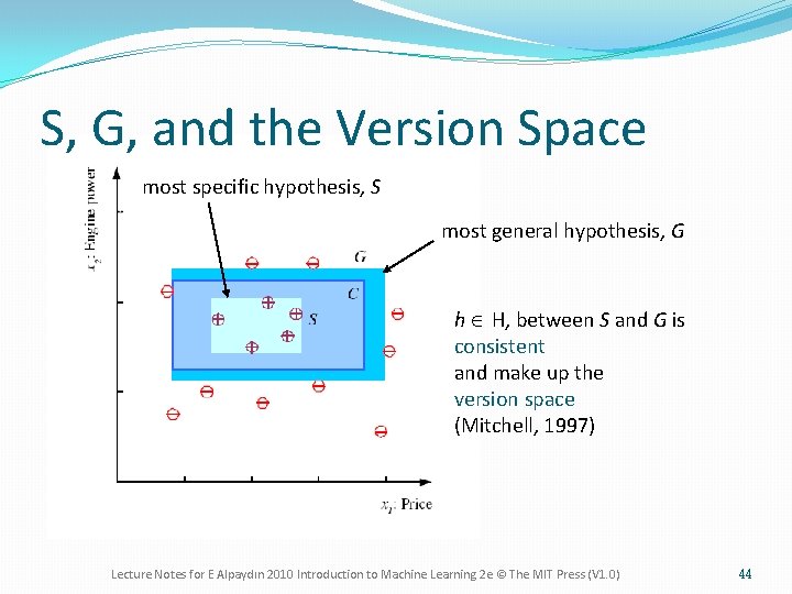
S, G, and the Version Space most specific hypothesis, S most general hypothesis, G h Î H, between S and G is consistent and make up the version space (Mitchell, 1997) Lecture Notes for E Alpaydın 2010 Introduction to Machine Learning 2 e © The MIT Press (V 1. 0) 44

Margin �Choose h with largest margin Lecture Notes for E Alpaydın 2010 Introduction to Machine Learning 2 e © The MIT Press (V 1. 0) 45

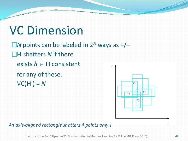
VC Dimension �N points can be labeled in 2 N ways as +/– �H shatters N if there exists h Î H consistent for any of these: VC(H ) = N An axis-aligned rectangle shatters 4 points only ! Lecture Notes for E Alpaydın 2010 Introduction to Machine Learning 2 e © The MIT Press (V 1. 0) 46

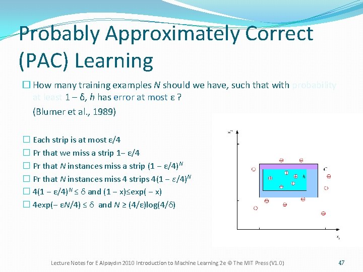
Probably Approximately Correct (PAC) Learning � How many training examples N should we have, such that with probability at least 1 ‒ δ, h has error at most ε ? (Blumer et al. , 1989) � Each strip is at most ε/4 � Pr that we miss a strip 1‒ ε/4 � Pr that N instances miss a strip (1 ‒ ε/4)N � Pr that N instances miss 4 strips 4(1 ‒ ε/4)N � 4(1 ‒ ε/4)N ≤ δ and (1 ‒ x)≤exp( ‒ x) � 4 exp(‒ εN/4) ≤ δ and N ≥ (4/ε)log(4/δ) Lecture Notes for E Alpaydın 2010 Introduction to Machine Learning 2 e © The MIT Press (V 1. 0) 47

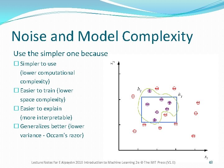
Noise and Model Complexity Use the simpler one because � Simpler to use (lower computational complexity) � Easier to train (lower space complexity) � Easier to explain (more interpretable) � Generalizes better (lower variance - Occam’s razor) Lecture Notes for E Alpaydın 2010 Introduction to Machine Learning 2 e © The MIT Press (V 1. 0) 48

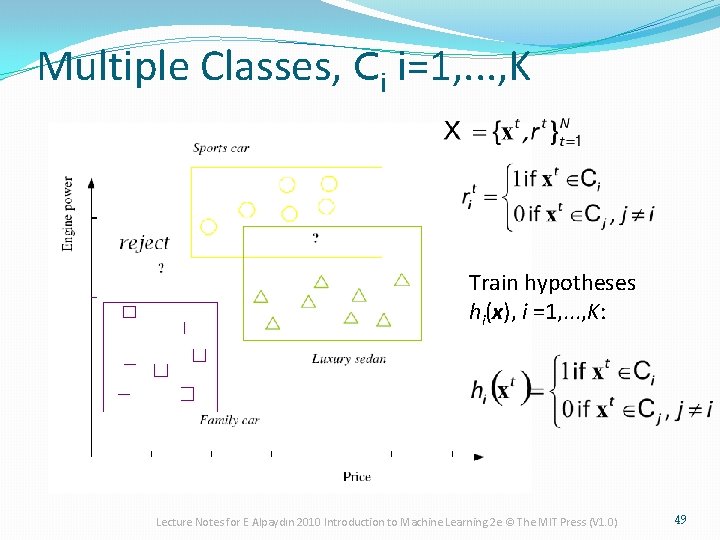
Multiple Classes, Ci i=1, . . . , K Train hypotheses hi(x), i =1, . . . , K: Lecture Notes for E Alpaydın 2010 Introduction to Machine Learning 2 e © The MIT Press (V 1. 0) 49

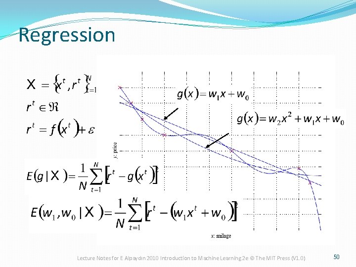
Regression Lecture Notes for E Alpaydın 2010 Introduction to Machine Learning 2 e © The MIT Press (V 1. 0) 50

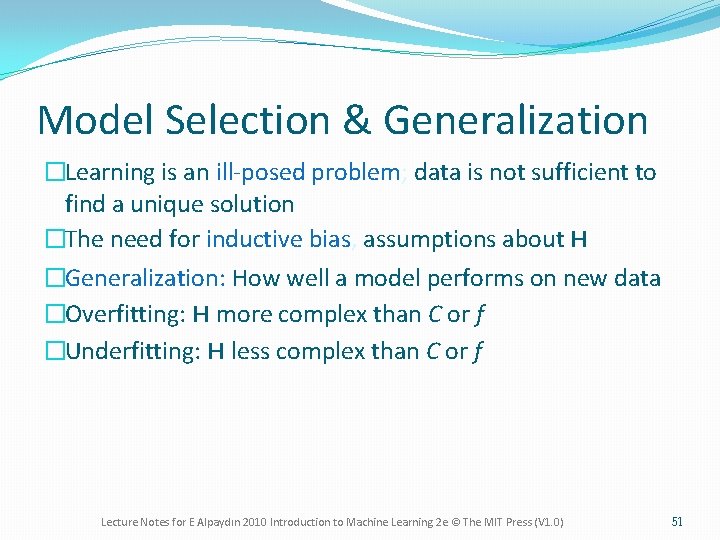
Model Selection & Generalization �Learning is an ill-posed problem; data is not sufficient to find a unique solution �The need for inductive bias, assumptions about H �Generalization: How well a model performs on new data �Overfitting: H more complex than C or f �Underfitting: H less complex than C or f Lecture Notes for E Alpaydın 2010 Introduction to Machine Learning 2 e © The MIT Press (V 1. 0) 51

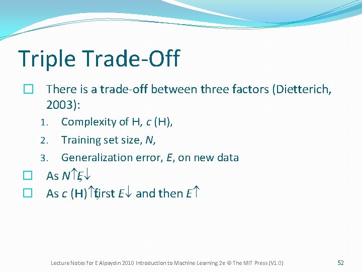
Triple Trade-Off � There is a trade-off between three factors (Dietterich, 2003): 1. Complexity of H, c (H), 2. Training set size, N, 3. Generalization error, E, on new data ¨ As N , E¯ ¨ As c (H) , first E¯ and then E Lecture Notes for E Alpaydın 2010 Introduction to Machine Learning 2 e © The MIT Press (V 1. 0) 52

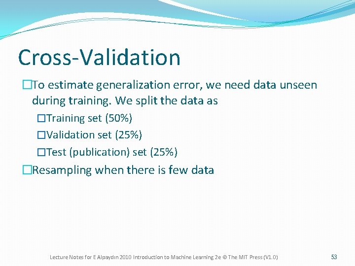
Cross-Validation �To estimate generalization error, we need data unseen during training. We split the data as �Training set (50%) �Validation set (25%) �Test (publication) set (25%) �Resampling when there is few data Lecture Notes for E Alpaydın 2010 Introduction to Machine Learning 2 e © The MIT Press (V 1. 0) 53

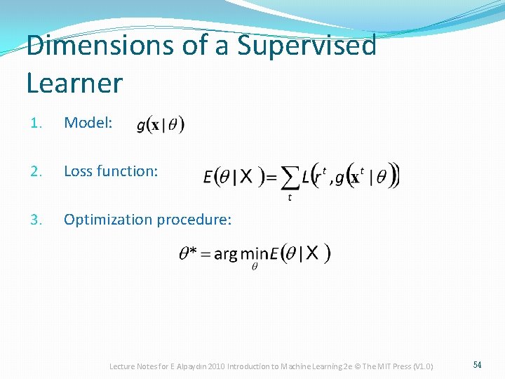
Dimensions of a Supervised Learner 1. Model: 2. Loss function: 3. Optimization procedure: Lecture Notes for E Alpaydın 2010 Introduction to Machine Learning 2 e © The MIT Press (V 1. 0) 54