Machine Learning Octave tutorial 2016 3 15 Octave

Machine Learning Octave tutorial 2016. 3. 15 데이터 마이닝 박영택

Octave Tutorial Basic operations Machine Learning

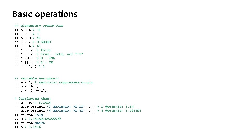
Basic operations %% >> >> >> elementary operations 5 + 6 % 11 3 - 2 % 1 5 * 8 % 40 1 / 2 % 0. 50000 2 ^ 6 % 64 1 == 2 % false 1 ~= 2 % true. note, not "!=" 1 && 0 % 0 : AND 1 || 0 % 1 : OR xor(1, 0) % 1 %% >> >> >> variable assignment a = 3; % semicolon suppresses output b = 'hi'; c = (3 >= 1); % Displaying them: >> a = pi % 3. 1416 >> disp(sprintf('2 decimals: %0. 2 f', a)) % 2 decimals: 3. 14 >> disp(sprintf('6 decimals: %0. 6 f', a)) % 6 decimals: 3. 141593 >> format long >> a % 3. 14159265358979 >> format short >> a % 3. 1416

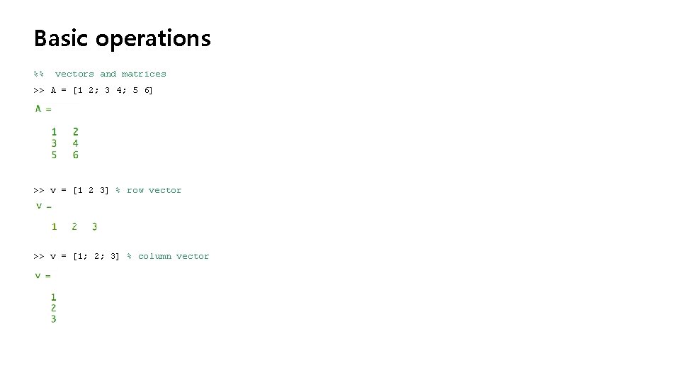
Basic operations %% vectors and matrices >> A = [1 2; 3 4; 5 6] >> v = [1 2 3] % row vector >> v = [1; 2; 3] % column vector

Basic operations >> v = [1: 0. 1: 2] % from 1 to 2, with step size of 0. 1. Useful for plot axes >> v = 1: 6 % from 1 to 6, assumes step size of 1 >> C = 2*ones(2, 3) % same as C = [2 2 2; 2 2 2]

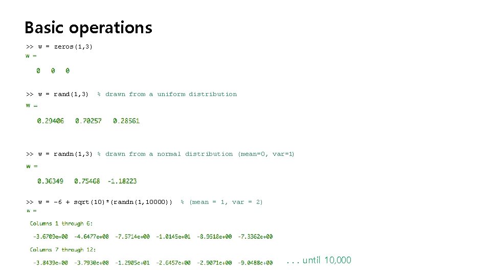
Basic operations >> w = zeros(1, 3) >> w = rand(1, 3) % drawn from a uniform distribution >> w = randn(1, 3) % drawn from a normal distribution (mean=0, var=1) >> w = -6 + sqrt(10)*(randn(1, 10000)) % (mean = 1, var = 2) . . . until 10, 000

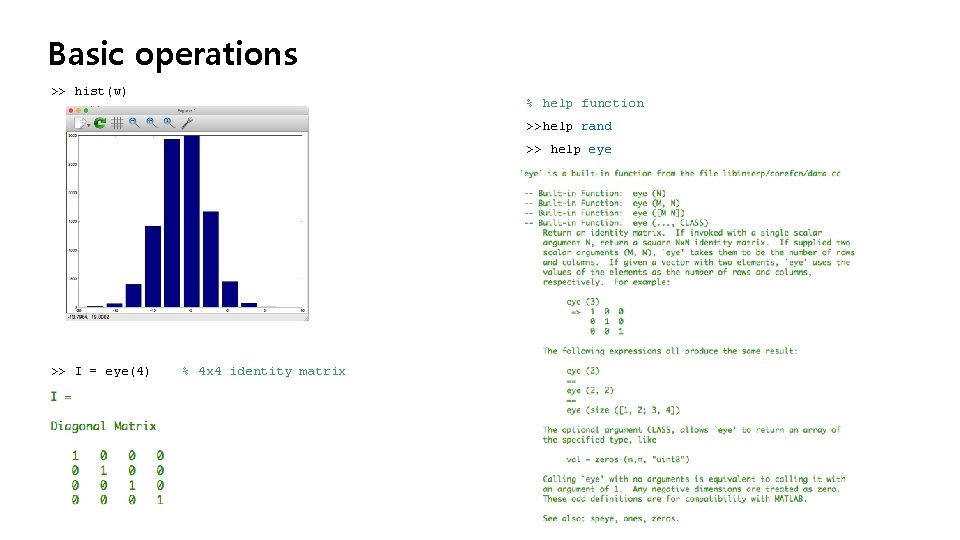
Basic operations >> hist(w) % help function >>help rand >> help eye >> I = eye(4) % 4 x 4 identity matrix

Octave Tutorial Moving data around Machine Learning

Moving data around %% dimensions >> A = [1 2; 3 4; 5 6] >> sz = size(A) >> size(A, 1) % number of rows >> size(A, 2) % number of cols >> length(sz) % size of longest dimension

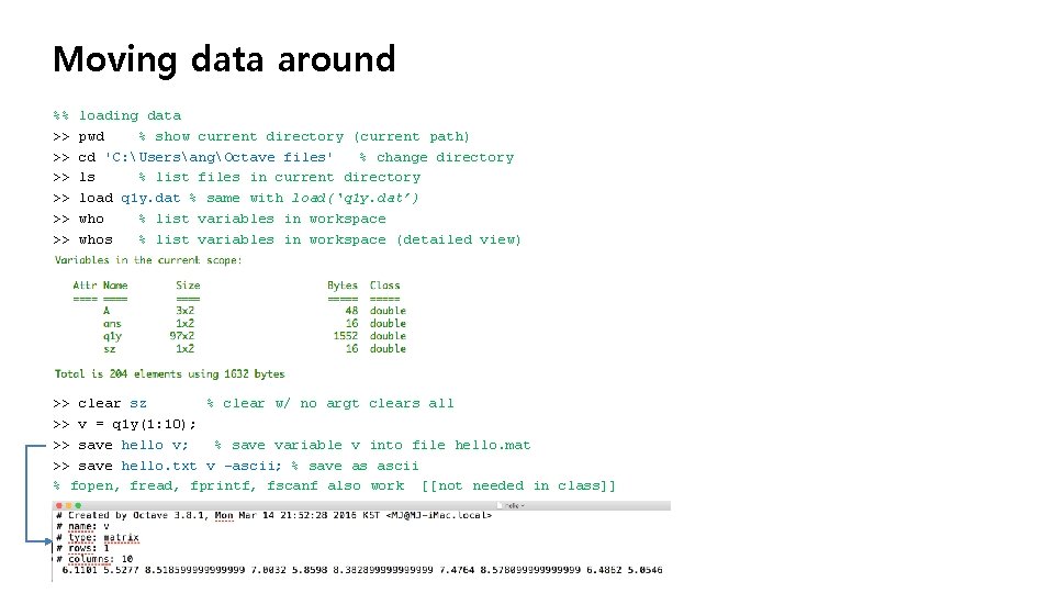
Moving data around %% >> >> >> loading data pwd % show current directory (current path) cd 'C: UsersangOctave files' % change directory ls % list files in current directory load q 1 y. dat % same with load(‘q 1 y. dat’) who % list variables in workspace whos % list variables in workspace (detailed view) >> clear sz % clear w/ no argt clears all >> v = q 1 y(1: 10); >> save hello v; % save variable v into file hello. mat >> save hello. txt v -ascii; % save as ascii % fopen, fread, fprintf, fscanf also work [[not needed in class]]

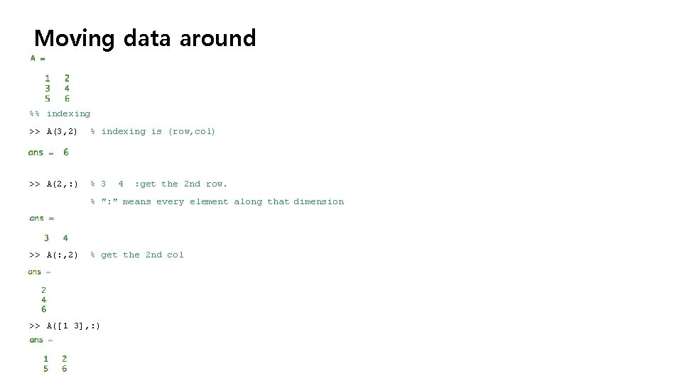
Moving data around %% indexing >> A(3, 2) % indexing is (row, col) >> A(2, : ) % 3 4 : get the 2 nd row. % ": " means every element along that dimension >> A(: , 2) % get the 2 nd col >> A([1 3], : )

Moving data around >> A(: , 2) = [10; 11; 12] % change second column >> A = [A, [100; 101; 102]] % append column vec >> A(: ) % Select all elements as a column vector.

Moving data around >> A = [1 2; 3 4; 5 6] >> B = [11 12; 13 14; 15 16] % same dims as A >> [A B] >> [A; B]

Octave Tutorial Computing on data Machine Learning

Computing on data >> A = [1 2; 3 4; 5 6] >> A * C % matrix multiplication >> B = [11 12; 13 14; 15 16] >> A. * B % element-wise multiplcation % A. * C or A * B gives error - wrong dimensions >> C = [1 1; 2 2] >> A. ^ 2

Computing on data >> V = [1; 2; 3] >> exp(V) % e^4 >> 1. / V >> -V % -1*v >> log(V) % functions like this operate element-wise on vecs or matrices >> abs(V) >> V + ones(length(V), 1) % v + 1 % same >> A' % matrix transpose if A is * A = (A’)’

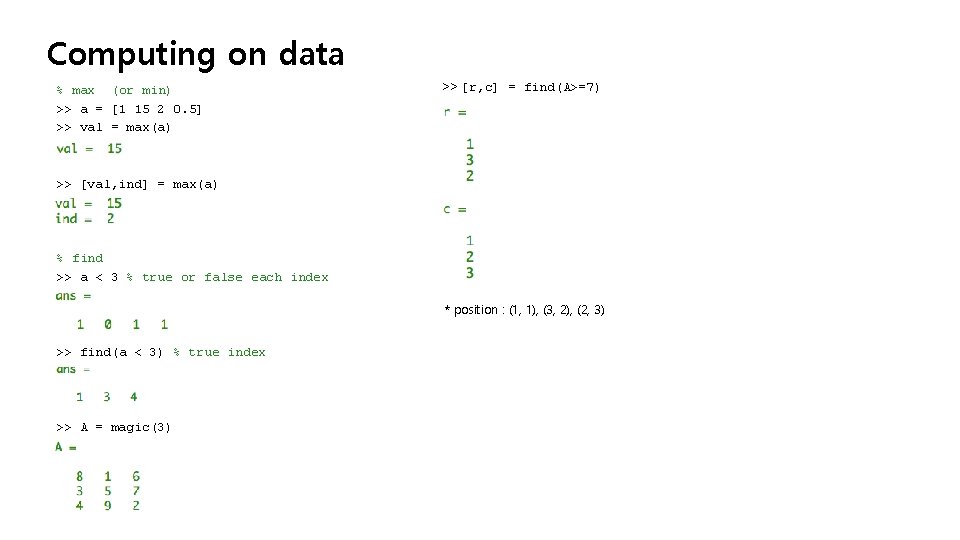
Computing on data % max (or min) >> a = [1 15 2 0. 5] >> val = max(a) >> [r, c] = find(A>=7) >> [val, ind] = max(a) % find >> a < 3 % true or false each index * position : (1, 1), (3, 2), (2, 3) >> find(a < 3) % true index >> A = magic(3)

Computing on data >> a = [1 15 2 0. 5]; >> sum(a) >> prod(a) % product >> max(A, [], 1) % max of column and same with max(A) >> floor(a) % down decimal or ceil(a) is up >> min(A, [], 2) % min of row >> max(rand(3), rand(3))

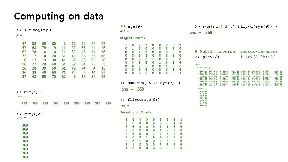
Computing on data >> A = magic(9) >> eye(9) >> sum( A. * flipud(eye(9)) )) % Matrix inverse (pseudo-inverse) >> pinv(A) % inv(A'*A)*A' >> sum( A. * eye(9) )) >> sum(A, 1) >> flipud(eye(9)) >> sum(A, 2)

Octave Tutorial Plotting data Machine Learning

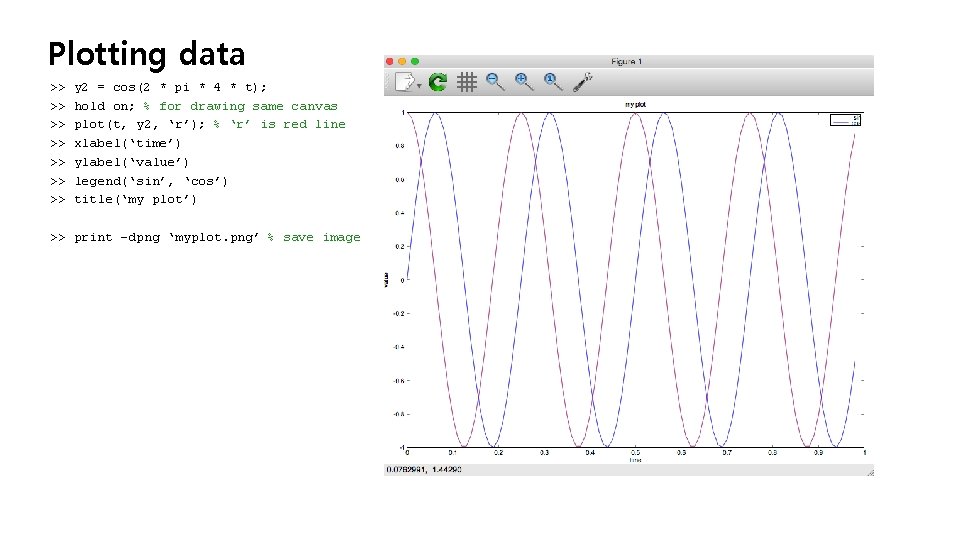
Plotting data >> t = [0: 0. 01: 0. 98]; >> y 1 = sin(2 * pi * 4 * t); >> plot(t, y 1); >> y 2 = cos(2 * pi * 4 * t); >> hold on; % for drawing same canvas >> plot(t, y 2, ‘r’); % ‘r’ is red line

Plotting data >> >> y 2 = cos(2 * pi * 4 * t); hold on; % for drawing same canvas plot(t, y 2, ‘r’); % ‘r’ is red line xlabel(‘time’) ylabel(‘value’) legend(‘sin’, ‘cos’) title(‘my plot’) >> print –dpng ‘myplot. png’ % save image

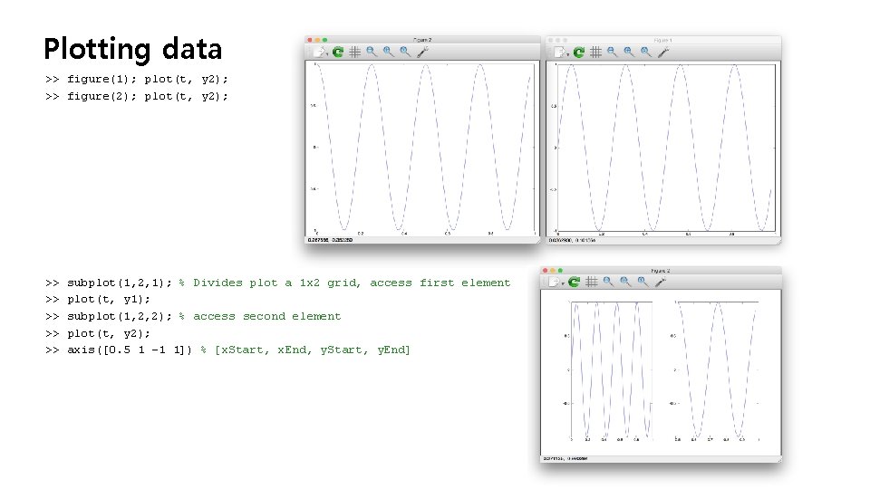
Plotting data >> figure(1); plot(t, y 2); >> figure(2); plot(t, y 2); >> >> >> subplot(1, 2, 1); % Divides plot a 1 x 2 grid, access first element plot(t, y 1); subplot(1, 2, 2); % access second element plot(t, y 2); axis([0. 5 1 -1 1]) % [x. Start, x. End, y. Start, y. End]

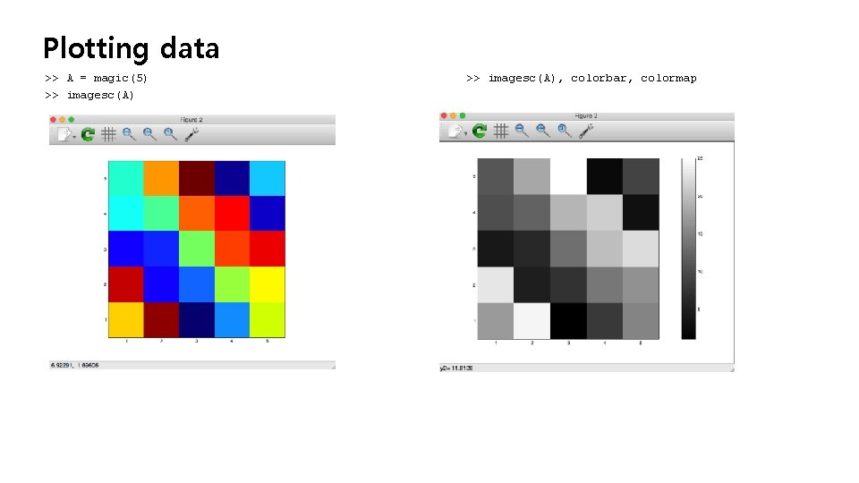
Plotting data >> A = magic(5) >> imagesc(A), colorbar, colormap

Octave Tutorial Control statements: for, while, if statements Machine Learning

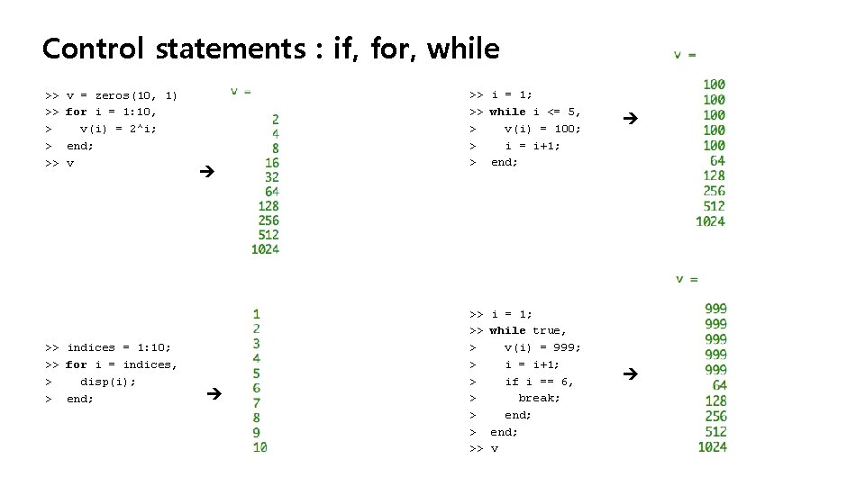
Control statements : if, for, while >> >> > > >> v = zeros(10, 1) for i = 1: 10, v(i) = 2^i; end; v >> indices = 1: 10; >> for i = indices, > disp(i); > end; >> i = 1; >> while i <= 5, > v(i) = 100; > i = i+1; > end; >> >> > > > >> i = 1; while true, v(i) = 999; i = i+1; if i == 6, break; end; v

Control statements : function >> function [y 1, y 2] = square. And. Cube. This. Number(x) > y 1 = x^2; > y 2 = x^3; > end; >> [q, w] = square. And. Cube. This. Number(3) % can have 2 return values q = 9 w = 27

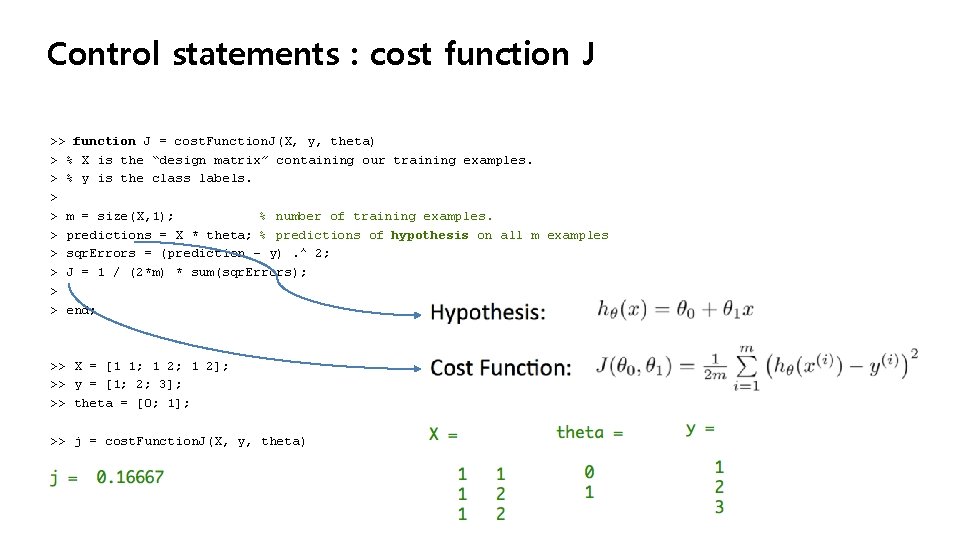
Control statements : cost function J >> function J = cost. Function. J(X, y, theta) > % X is the “design matrix” containing our training examples. > % y is the class labels. > > m = size(X, 1); % number of training examples. > predictions = X * theta; % predictions of hypothesis on all m examples > sqr. Errors = (prediction – y). ^ 2; > J = 1 / (2*m) * sum(sqr. Errors); > > end; >> X = [1 1; 1 2]; >> y = [1; 2; 3]; >> theta = [0; 1]; >> j = cost. Function. J(X, y, theta)

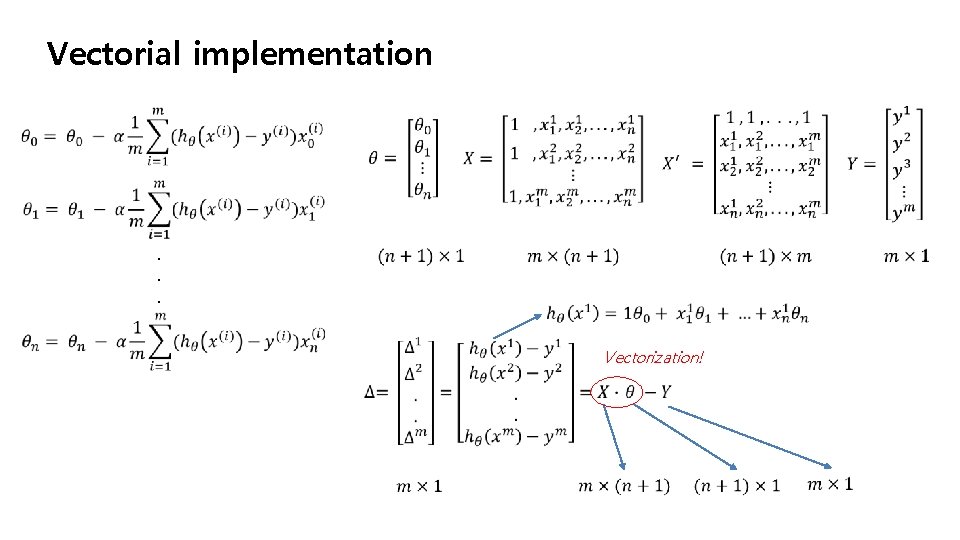
Octave Tutorial Vectorial implementation Machine Learning

Vectorial implementation . . . Vectorization!

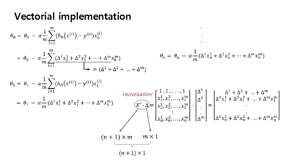
Vectorial implementation. . . Vectorization!

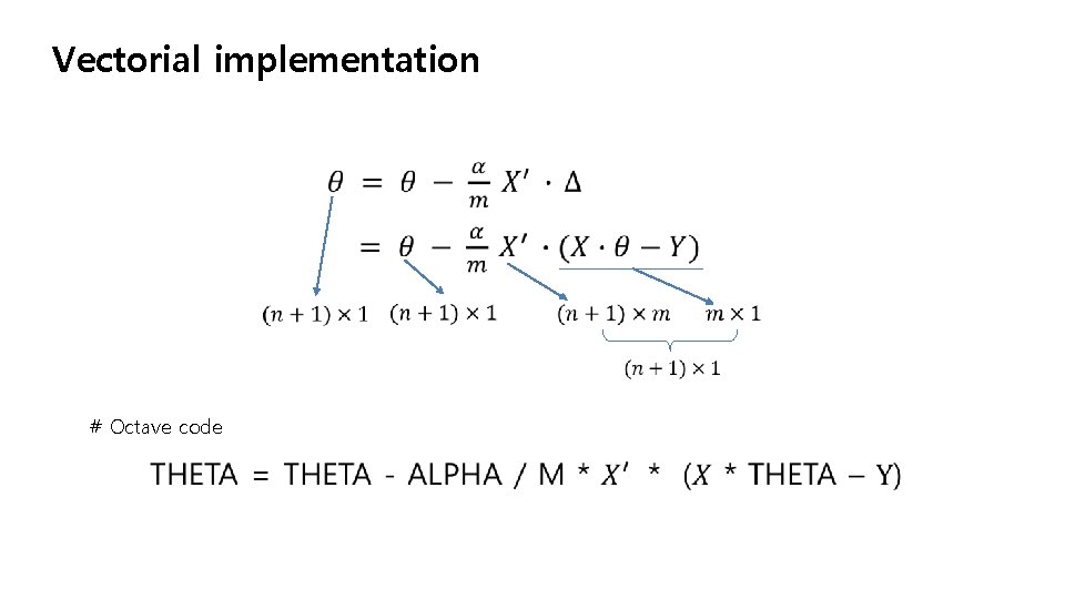
Vectorial implementation # Octave code