Machine Learning Introduction CSE 4309 Machine Learning Vassilis
- Slides: 46

Machine Learning - Introduction CSE 4309 – Machine Learning Vassilis Athitsos Computer Science and Engineering Department University of Texas at Arlington 1

What is Machine Learning • Quote by Tom M. Mitchell: "A computer program is said to learn from experience E with respect to some class of tasks T and performance measure P if its performance at tasks in T, as measured by P, improves with experience E. " • To define a machine learning problem, we need to specify: – The experience (usually known as training data). – The task (classification, regression, …) – The performance measure (classification accuracy, squared error, …). 2

Types of Machine Learning (source: Wikipedia) • Supervised Learning. – The computer is presented with example inputs and their desired outputs, given by a "teacher", and the goal is to learn a general rule that maps inputs to outputs. • Unsupervised Learning. – No example outputs are given to the learning algorithm, leaving it on its own to find structure in its input. • Reinforcement Learning. – A computer program interacts with a dynamic environment and must perform a certain goal (such as driving a car or playing chess). The program is provided feedback (rewards and 3 punishments).

Supervised Learning • The computer is presented with example inputs and their desired outputs, given by a "teacher". • Goal: learn a general function that maps inputs to outputs.

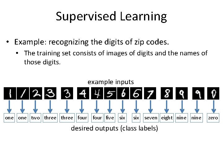
Supervised Learning • Example: recognizing the digits of zip codes. • The training set consists of images of digits and the names of those digits. example inputs one two three four five six seven eight nine desired outputs (class labels) zero

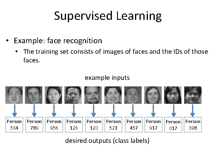
Supervised Learning • Example: face recognition • The training set consists of images of faces and the IDs of those faces. example inputs Person Person Person 534 789 956 120 521 457 917 398 017 desired outputs (class labels)

Regression, Classification, Pattern Recognition • When the desired output belongs to one of a finite number of categories, then the supervised learning problem is called a classification problem. • When the desired output contains one or more values from a continuous space, then the supervised learning problem is called a regression problem. 7

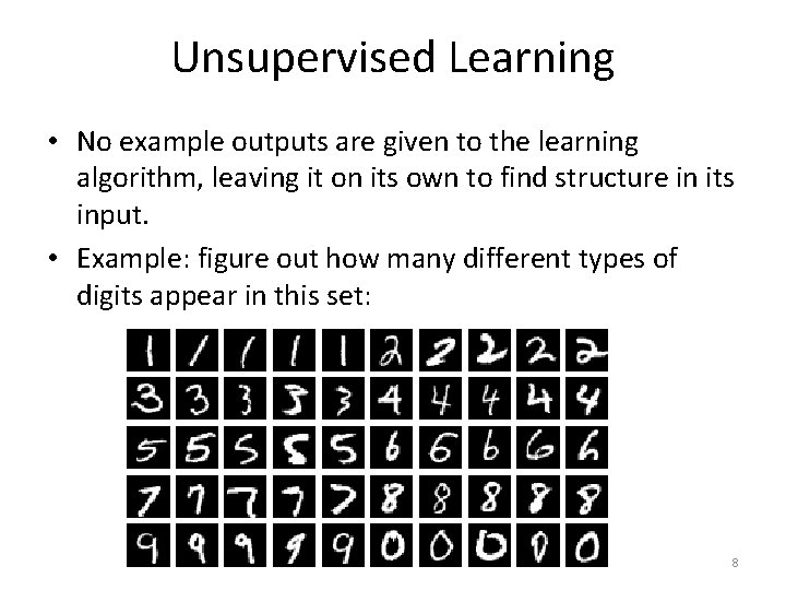
Unsupervised Learning • No example outputs are given to the learning algorithm, leaving it on its own to find structure in its input. • Example: figure out how many different types of digits appear in this set: 8

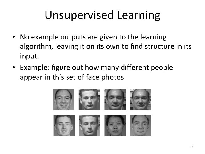
Unsupervised Learning • No example outputs are given to the learning algorithm, leaving it on its own to find structure in its input. • Example: figure out how many different people appear in this set of face photos: 9

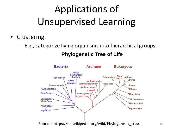
Applications of Unsupervised Learning • Clustering. – E. g. , categorize living organisms into hierarchical groups. Source: https: //en. wikipedia. org/wiki/Phylogenetic_tree 10

Applications of Unsupervised Learning • Anomaly detection. – Figure out if someone at an airport is behaving abnormally, which may be a sign of danger. – Figure out if an engine is behaving abnormally, which may be a sign of malfunction/damage. • This can also be treated as a supervised learning problem, if someone provides training examples that are labeled as "anomalies". • If it is treated as an unsupervised learning problem, then an anomaly model must be built without such 11 training examples.

Reinforcement Learning • Learn what actions to take so as to maximize reward. • Correct pairs of input/output are not presented to the system. • The system needs to explore different actions at different situations, to see what rewards it gets. • However, the system also needs to exploit its knowledge so as to maximize rewards. – Problem: what is the optimal balance between exploration and exploitation? 12

Applications of Reinforcement Learning • A robot learning how to move a robotic arm, or how to walk on two legs. • A car learning how to drive itself. • A computer program learning how to play a board game, like chess, tic-tac-toe, etc. 13

Machine Learning and Pattern Recognition • Machine learning and pattern recognition are not the same thing. – This is a point that confuses many people. • You can use machine learning to learn things that are not classifiers. For example: – Learn how to walk on two feet. – Learn how to grasp a medical tool. • You can construct classifiers without machine learning. – You can hardcode a bunch of rules that the classifier applies to each pattern in order to estimate its class. • However, machine learning and pattern recognition are heavily related. – A big part of machine learning research focuses on pattern recognition. – Modern pattern recognition systems are usually exclusively based on machine learning. 14

Topics for This Semester • Main emphasis: supervised learning. • We will study several different approaches: – – – – Bayesian classifiers. Neural networks. Kernel methods and support vector machines. Nearest neighbors. Boosting. Decision trees. Graphical models. • Towards the end, we will briefly study unsupervised learning and reinforcement learning. 15

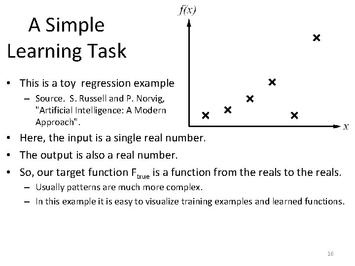
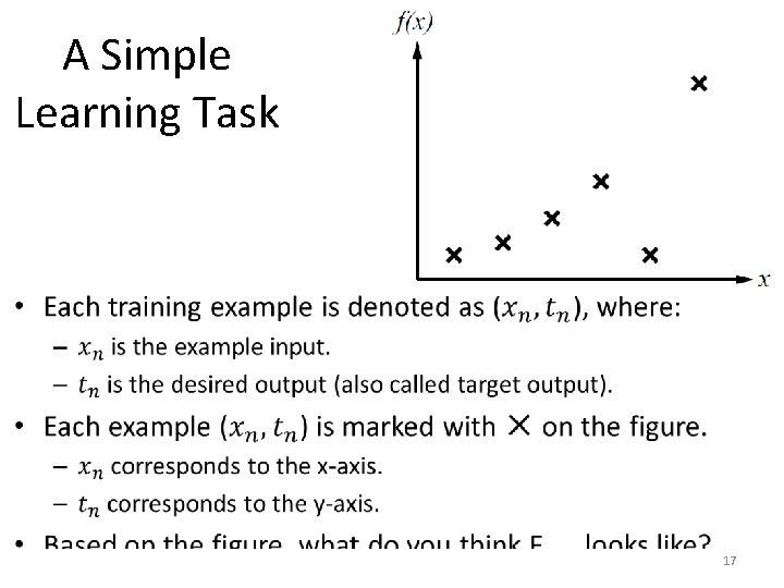
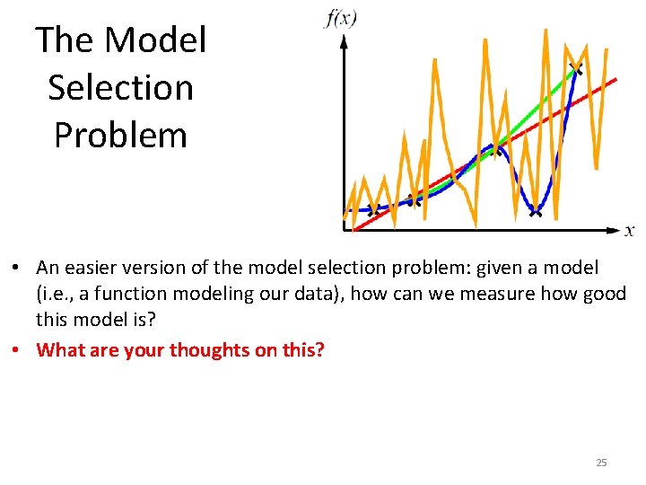
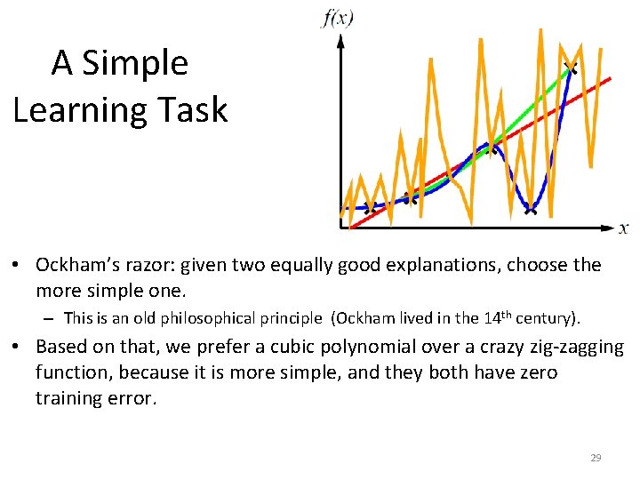
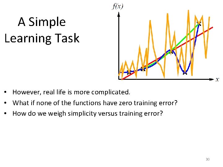
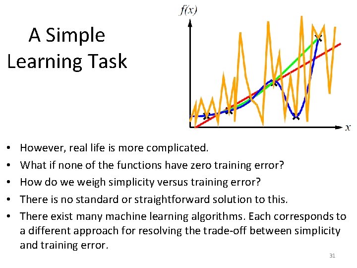
A Simple Learning Task • This is a toy regression example. . – Source. S. Russell and P. Norvig, "Artificial Intelligence: A Modern Approach". • Here, the input is a single real number. • The output is also a real number. • So, our target function Ftrue is a function from the reals to the reals. – Usually patterns are much more complex. – In this example it is easy to visualize training examples and learned functions. 16

A Simple Learning Task • 17

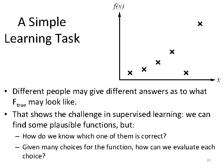
A Simple Learning Task • Different people may give different answers as to what Ftrue may look like. • That shows the challenge in supervised learning: we can find some plausible functions, but: – How do we know which one of them is correct? – Given many choices for the function, how can we evaluate each choice? 18

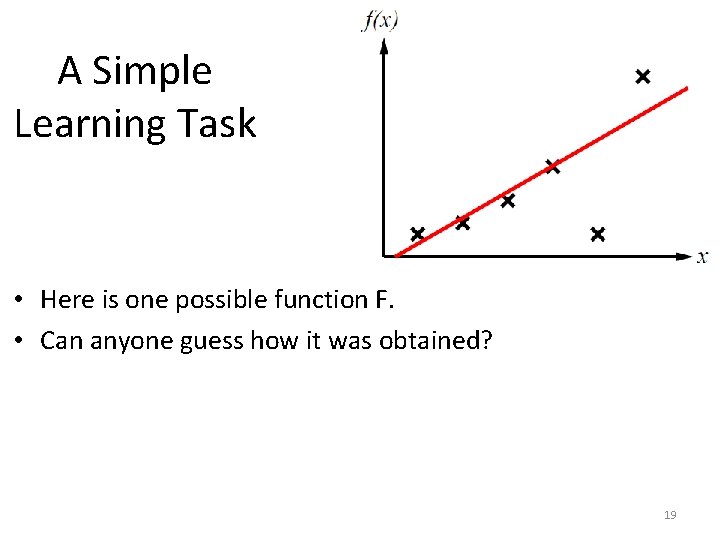
A Simple Learning Task • Here is one possible function F. • Can anyone guess how it was obtained? 19

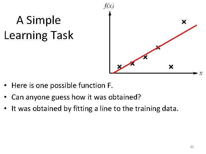
A Simple Learning Task • Here is one possible function F. • Can anyone guess how it was obtained? • It was obtained by fitting a line to the training data. 20

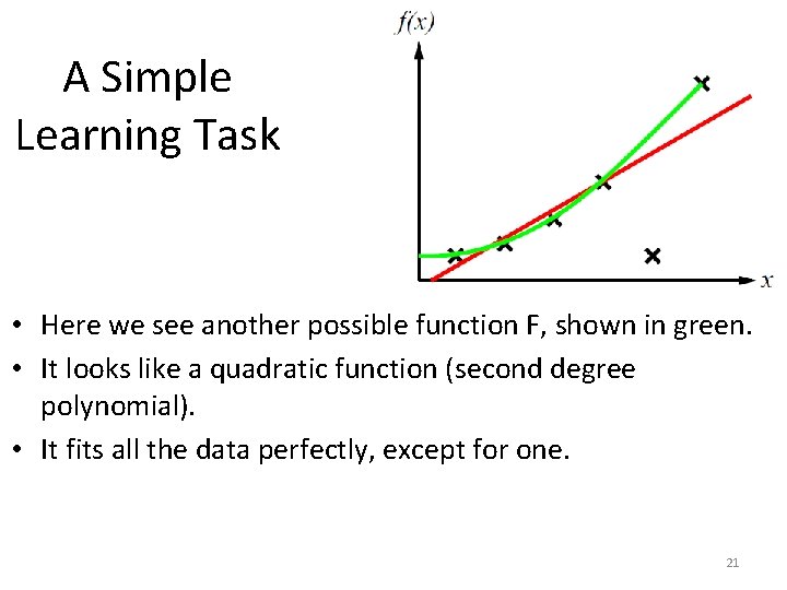
A Simple Learning Task • Here we see another possible function F, shown in green. • It looks like a quadratic function (second degree polynomial). • It fits all the data perfectly, except for one. 21

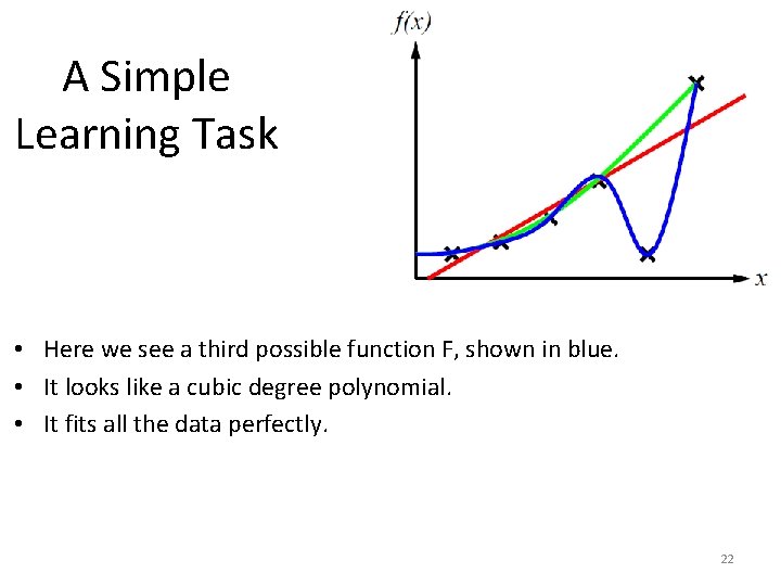
A Simple Learning Task • Here we see a third possible function F, shown in blue. • It looks like a cubic degree polynomial. • It fits all the data perfectly. 22

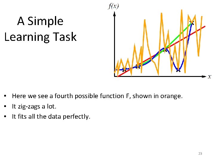
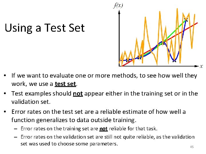
A Simple Learning Task • Here we see a fourth possible function F, shown in orange. • It zig-zags a lot. • It fits all the data perfectly. 23

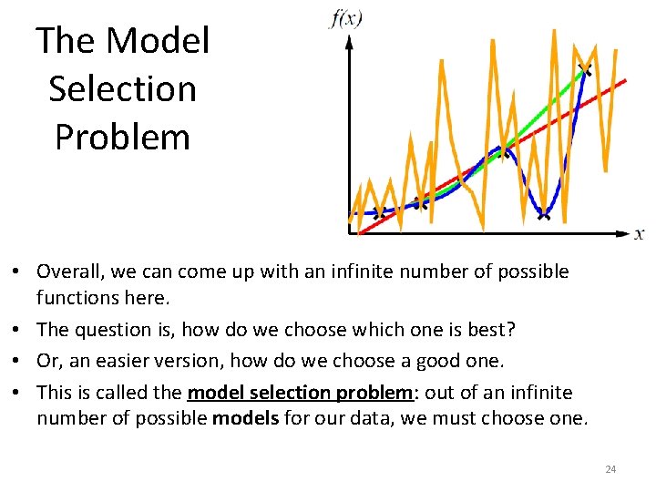
The Model Selection Problem • Overall, we can come up with an infinite number of possible functions here. • The question is, how do we choose which one is best? • Or, an easier version, how do we choose a good one. • This is called the model selection problem: out of an infinite number of possible models for our data, we must choose one. 24

The Model Selection Problem • An easier version of the model selection problem: given a model (i. e. , a function modeling our data), how can we measure how good this model is? • What are your thoughts on this? 25

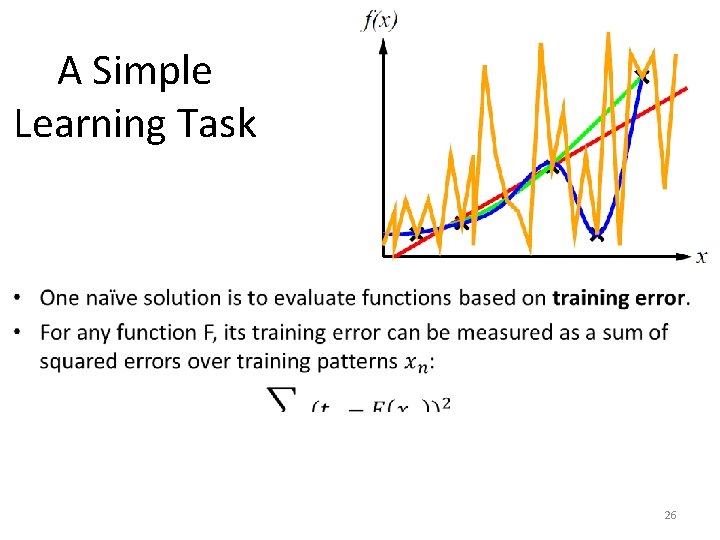
A Simple Learning Task • 26

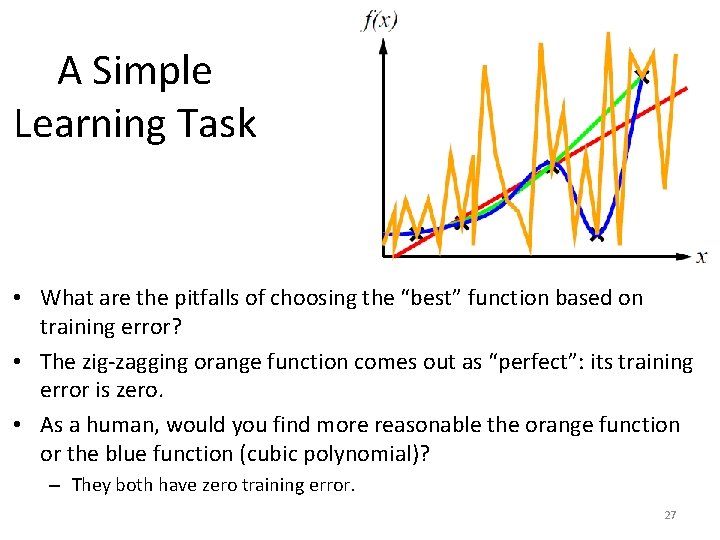
A Simple Learning Task • What are the pitfalls of choosing the “best” function based on training error? • The zig-zagging orange function comes out as “perfect”: its training error is zero. • As a human, would you find more reasonable the orange function or the blue function (cubic polynomial)? – They both have zero training error. 27

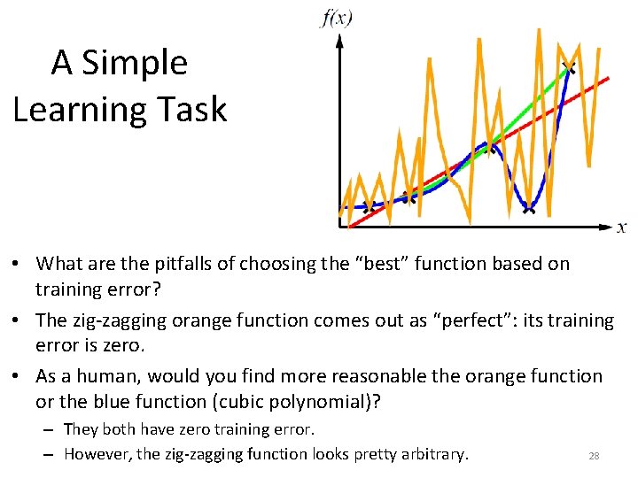
A Simple Learning Task • What are the pitfalls of choosing the “best” function based on training error? • The zig-zagging orange function comes out as “perfect”: its training error is zero. • As a human, would you find more reasonable the orange function or the blue function (cubic polynomial)? – They both have zero training error. – However, the zig-zagging function looks pretty arbitrary. 28

A Simple Learning Task • Ockham’s razor: given two equally good explanations, choose the more simple one. – This is an old philosophical principle (Ockham lived in the 14 th century). • Based on that, we prefer a cubic polynomial over a crazy zig-zagging function, because it is more simple, and they both have zero training error. 29

A Simple Learning Task • However, real life is more complicated. • What if none of the functions have zero training error? • How do we weigh simplicity versus training error? 30

A Simple Learning Task • • • However, real life is more complicated. What if none of the functions have zero training error? How do we weigh simplicity versus training error? There is no standard or straightforward solution to this. There exist many machine learning algorithms. Each corresponds to a different approach for resolving the trade-off between simplicity and training error. 31

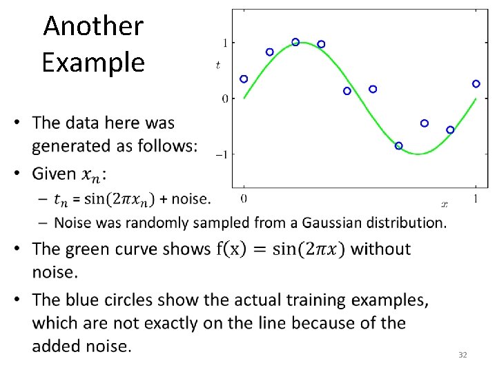
Another Example • 32

Polynomial Fitting • 33

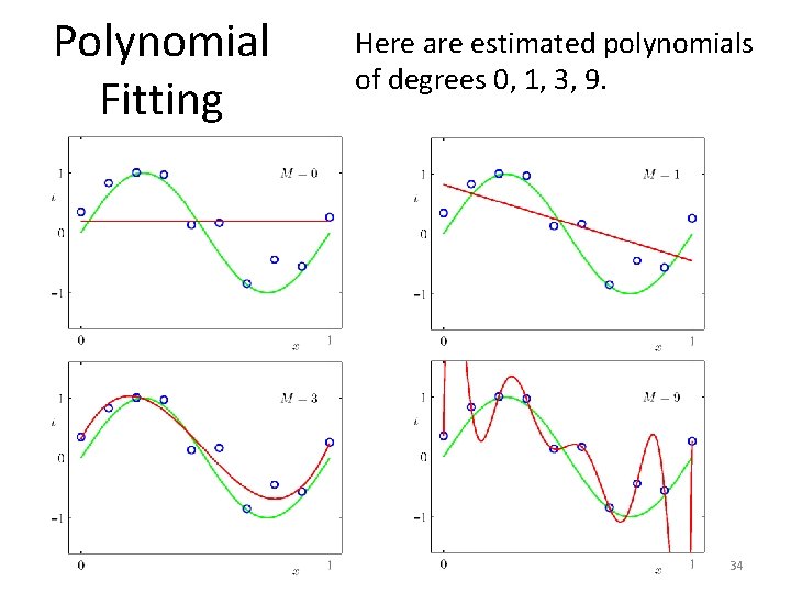
Polynomial Fitting Here are estimated polynomials of degrees 0, 1, 3, 9. 34

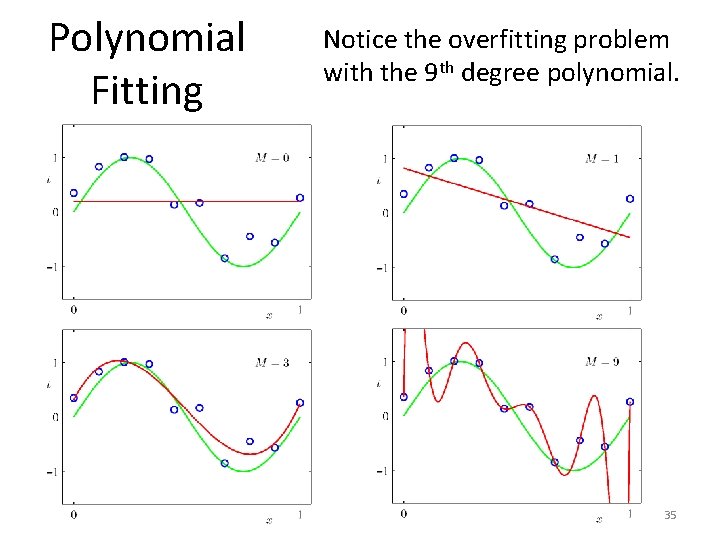
Polynomial Fitting Notice the overfitting problem with the 9 th degree polynomial. 35

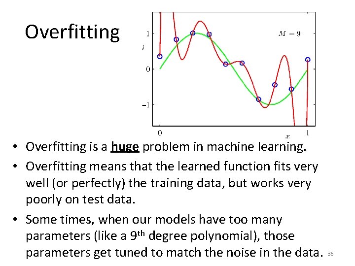
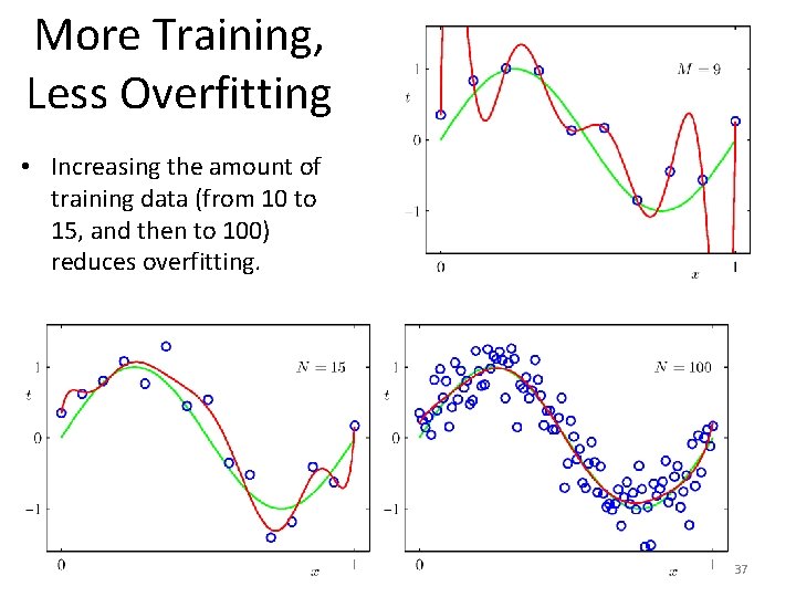
Overfitting • Overfitting is a huge problem in machine learning. • Overfitting means that the learned function fits very well (or perfectly) the training data, but works very poorly on test data. • Some times, when our models have too many parameters (like a 9 th degree polynomial), those parameters get tuned to match the noise in the data. 36

More Training, Less Overfitting • Increasing the amount of training data (from 10 to 15, and then to 100) reduces overfitting. 37

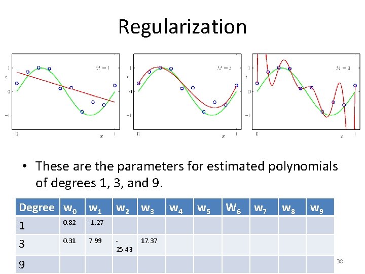
Regularization • These are the parameters for estimated polynomials of degrees 1, 3, and 9. Degree w 0 0. 82 1 0. 31 3 9 w 1 w 2 w 3 w 4 w 5 W 6 w 7 w 8 w 9 -1. 27 7. 99 25. 43 17. 37 38

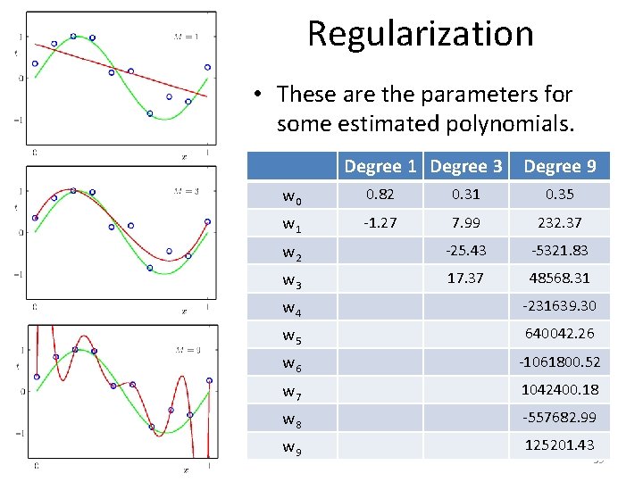
Regularization • These are the parameters for some estimated polynomials. Degree 1 Degree 3 Degree 9 w 0 0. 82 0. 31 0. 35 w 1 -1. 27 7. 99 232. 37 w 2 -25. 43 -5321. 83 w 3 17. 37 48568. 31 w 4 -231639. 30 w 5 640042. 26 w 6 -1061800. 52 w 7 1042400. 18 w 8 -557682. 99 w 9 125201. 43 39

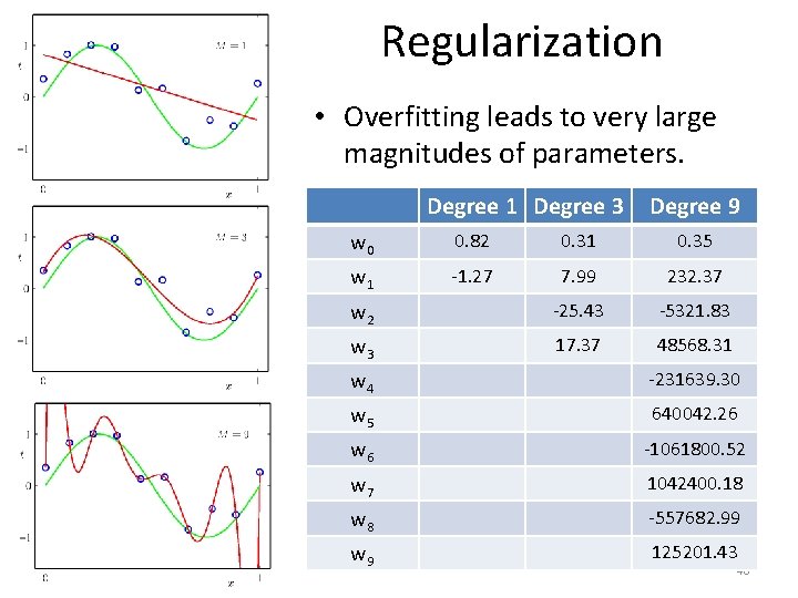
Regularization • Overfitting leads to very large magnitudes of parameters. Degree 1 Degree 3 Degree 9 w 0 0. 82 0. 31 0. 35 w 1 -1. 27 7. 99 232. 37 w 2 -25. 43 -5321. 83 w 3 17. 37 48568. 31 w 4 -231639. 30 w 5 640042. 26 w 6 -1061800. 52 w 7 1042400. 18 w 8 -557682. 99 w 9 125201. 43 40

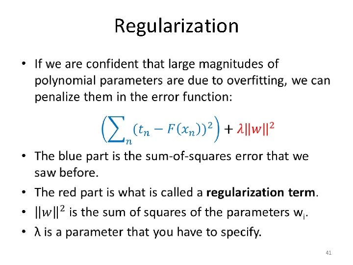
Regularization • 41

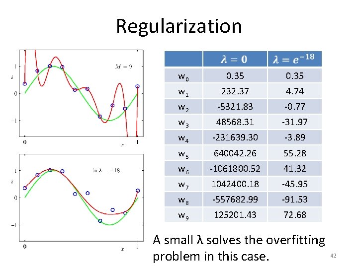
Regularization w 0 0. 35 w 1 232. 37 4. 74 w 2 -5321. 83 -0. 77 w 3 48568. 31 -31. 97 w 4 -231639. 30 -3. 89 w 5 640042. 26 55. 28 w 6 -1061800. 52 41. 32 w 7 1042400. 18 -45. 95 w 8 -557682. 99 -91. 53 w 9 125201. 43 72. 68 A small λ solves the overfitting 42 problem in this case.

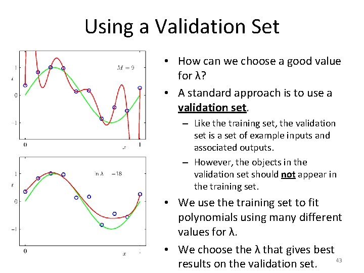
Using a Validation Set • How can we choose a good value for λ? • A standard approach is to use a validation set. – Like the training set, the validation set is a set of example inputs and associated outputs. – However, the objects in the validation set should not appear in the training set. • We use the training set to fit polynomials using many different values for λ. • We choose the λ that gives best 43 results on the validation set.

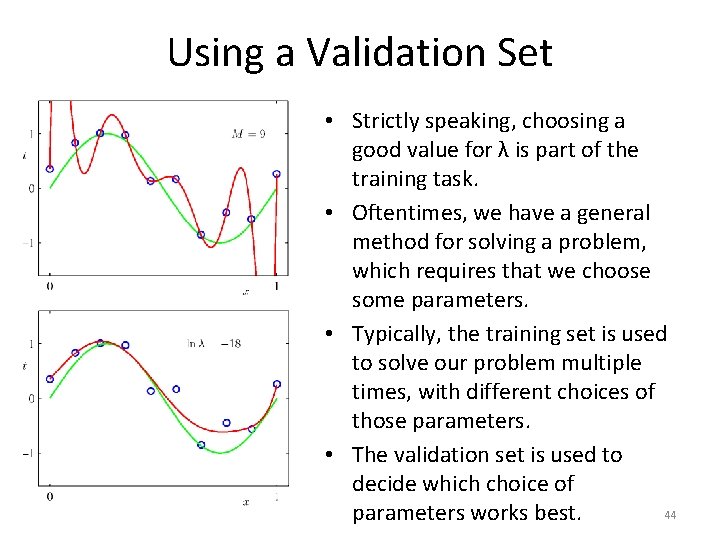
Using a Validation Set • Strictly speaking, choosing a good value for λ is part of the training task. • Oftentimes, we have a general method for solving a problem, which requires that we choose some parameters. • Typically, the training set is used to solve our problem multiple times, with different choices of those parameters. • The validation set is used to decide which choice of 44 parameters works best.

Using a Test Set • If we want to evaluate one or more methods, to see how well they work, we use a test set. • Test examples should not appear either in the training set or in the validation set. • Error rates on the test set are a reliable estimate of how well a function generalizes to data outside training. – Error rates on the training set are not reliable for that task. – Error rates on the validation set are still not quite reliable, as the validation set was used to choose some parameters. 45

Recap: Training, Validation, Test Sets • Training set: use to learn the function that we want to learn, that maps inputs to outputs. • Validation set: use to evaluate different values of parameters (like λ for regularization) that need to be hardcoded during training. – Train with different values, and then see how well each resulting function works on the validation set. • Test set: use to evaluate the final product (after the choice of parameters has been finalized). 46