Octave Tutorial Vectorial implementation Machine Learning Vectorial implementation


")
 Algorithm looks identical to linear")


 Advantages: Optimization")
![Example: function [j. Val, gradient] = cost. Function(theta) j. Val = (theta(1)-5)^2 +. .](https://slidetodoc.com/presentation_image_h2/441c3c50d75211213c5c87dc8a74a22c/image-11.jpg "Example: function [j. Val, gradient] = cost. Function(theta) j. Val = (theta(1)-5)^2 +. .")
![theta = function [j. Val, gradient] = cost. Function(theta) j. Val = [ code](https://slidetodoc.com/presentation_image_h2/441c3c50d75211213c5c87dc8a74a22c/image-12.jpg "theta = function [j. Val, gradient] = cost. Function(theta) j. Val = [ code")
; X = data(:")
![X = [ones(m, 1) X]; initial_theta = zeros(n + 1, 1); function g =](https://slidetodoc.com/presentation_image_h2/441c3c50d75211213c5c87dc8a74a22c/image-14.jpg "X = [ones(m, 1) X]; initial_theta = zeros(n + 1, 1); function g =")
![Logistic regression cost function [J, grad] = cost. Function(theta, X, y) m = length(y);](https://slidetodoc.com/presentation_image_h2/441c3c50d75211213c5c87dc8a74a22c/image-15.jpg "Logistic regression cost function [J, grad] = cost. Function(theta, X, y) m = length(y);")

![%% ======= Part 4: Predict and Accuracies ======= % prob = sigmoid([1 45 85]](https://slidetodoc.com/presentation_image_h2/441c3c50d75211213c5c87dc8a74a22c/image-19.jpg "%% ======= Part 4: Predict and Accuracies ======= % prob = sigmoid([1 45 85]")
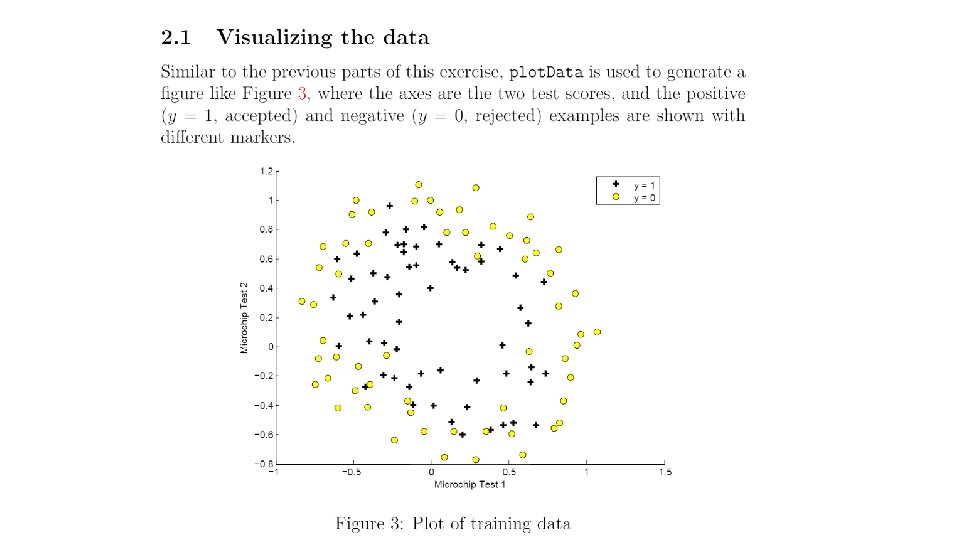
![data = load('ex 2 data 2. txt'); X = data(: , [1, 2]); y](https://slidetodoc.com/presentation_image_h2/441c3c50d75211213c5c87dc8a74a22c/image-22.jpg "data = load('ex 2 data 2. txt'); X = data(: , [1, 2]); y")
![Regularized linear regression function [J, grad] = cost. Function. Reg(theta, X, y, lambda) m](https://slidetodoc.com/presentation_image_h2/441c3c50d75211213c5c87dc8a74a22c/image-23.jpg "Regularized linear regression function [J, grad] = cost. Function. Reg(theta, X, y, lambda) m")
- Slides: 23
Octave Tutorial Vectorial implementation Machine Learning
Vectorial implementation . . . Vectorization!
Vectorial implementation. . . Vectorization!
Vectorial implementation # Octave code
Logistic regression cost function To fit parameters : To make a prediction given new Output :
Gradient Descent Want : Repeat (simultaneously update all )
Gradient Descent Want : Repeat (simultaneously update all ) Algorithm looks identical to linear regression!
Logistic Regression Advanced optimization Machine Learning
Optimization algorithm Cost function . Want Given , we have code that can compute (for ) Gradient descent: Repeat .
Optimization algorithm Given , we have code that can compute (for ) Advantages: Optimization algorithms: - No need to manually pick - Gradient descent - Conjugate gradient - Often faster than gradient - BFGS descent. - L-BFGS Disadvantages: - More complex
Example: function [j. Val, gradient] = cost. Function(theta) j. Val = (theta(1)-5)^2 +. . . (theta(2)-5)^2; gradient = zeros(2, 1); gradient(1) = 2*(theta(1)-5); gradient(2) = 2*(theta(2)-5); options = optimset(‘Grad. Obj’, ‘on’, ‘Max. Iter’, ‘ 100’); initial. Theta = zeros(2, 1); [opt. Theta, function. Val, exit. Flag]. . . = fminunc(@cost. Function, initial. Theta, options);
theta = function [j. Val, gradient] = cost. Function(theta) j. Val = [ code to compute gradient(1) = [ code to compute gradient(2) = [ code to compute gradient(n+1) = [ code to compute ]; ]; ];
Computer Cost and Gradient data = load('ex 2 data 1. txt'); X = data(: , [1, 2]); y = data(: , 3); [m, n] = size(X); X = [ones(m, 1) X]; initial_theta = zeros(n + 1, 1); % Compute and display initial cost and gradient [cost, grad] = cost. Function(initial_theta, X, y);
X = [ones(m, 1) X]; initial_theta = zeros(n + 1, 1); function g = sigmoid(z) g = 1. / (1 + exp(-1 * z)) ; End h = sigmoid(X * theta)
Logistic regression cost function [J, grad] = cost. Function(theta, X, y) m = length(y); % number of training examples % size(y) = m, 1 % size(X) = m, n+1 % size(theta) = n+1, 1 % size(h) = size(X * theta) = m, 1 J = 0; grad = zeros(size(theta)); h = sigmoid(X * theta); J = (1 / m) * (-y' * log(h) - (1 - y') * log(1 - h)) ; grad = (1 / m) * ( X * (h – y)) ; end
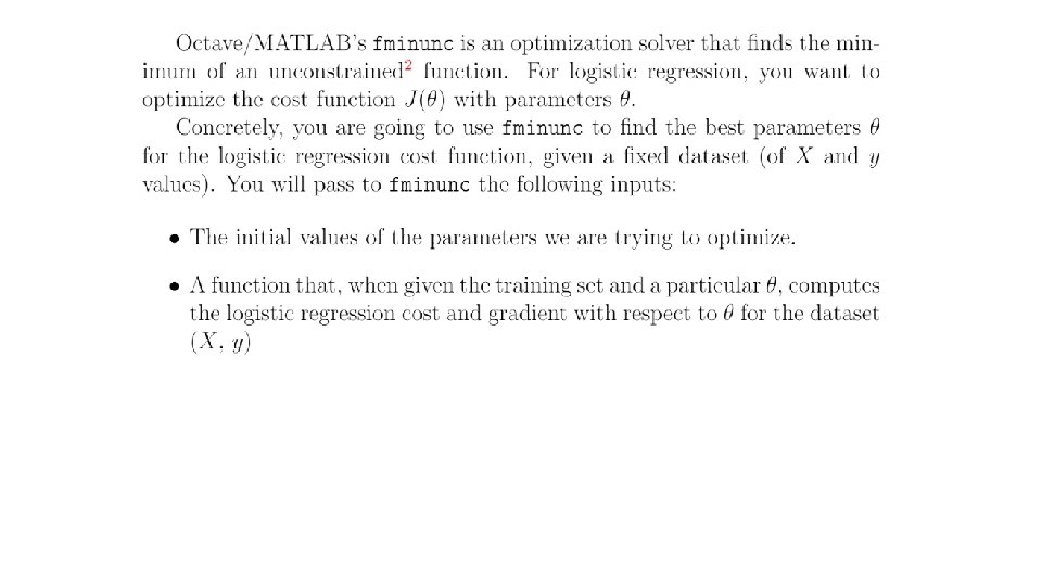
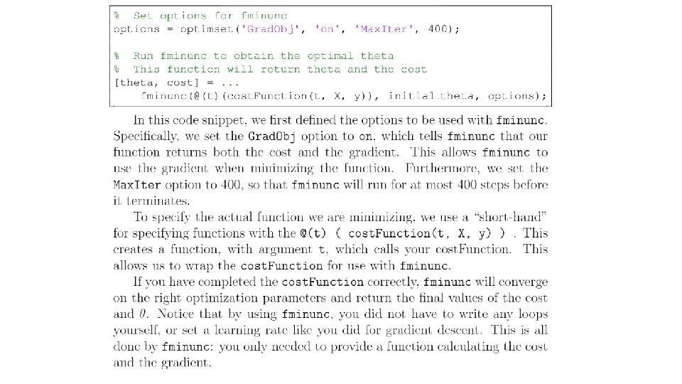
%% ======= Part 3: Optimizing using fminunc ======= % In this exercise, you will use a built-in function (fminunc) to find the % optimal parameters theta. % Set options for fminunc options = optimset('Grad. Obj', 'on', 'Max. Iter', 400); % Run fminunc to obtain the optimal theta % This function will return theta and the cost [theta, cost] =. . . fminunc(@(t)(cost. Function(t, X, y)), initial_theta, options); % Print theta to screen fprintf('Cost at theta found by fminunc: %fn', cost); fprintf('theta: n'); fprintf(' %f n', theta); % Plot Boundary plot. Decision. Boundary(theta, X, y);
%% ======= Part 4: Predict and Accuracies ======= % prob = sigmoid([1 45 85] * theta); fprintf(['For a student with scores 45 and 85, we predict an admission '. . . 'probability of %fnn'], prob); % Compute accuracy on our training set p = predict(theta, X); fprintf('Train Accuracy: %fn', mean(double(p == y)) * 100); function p = predict(theta, X) m = size(X, 1); % Number of training examples p = zeros(m, 1); h = sigmoid(x * theta) ; p = h >= 0. 5 ; end
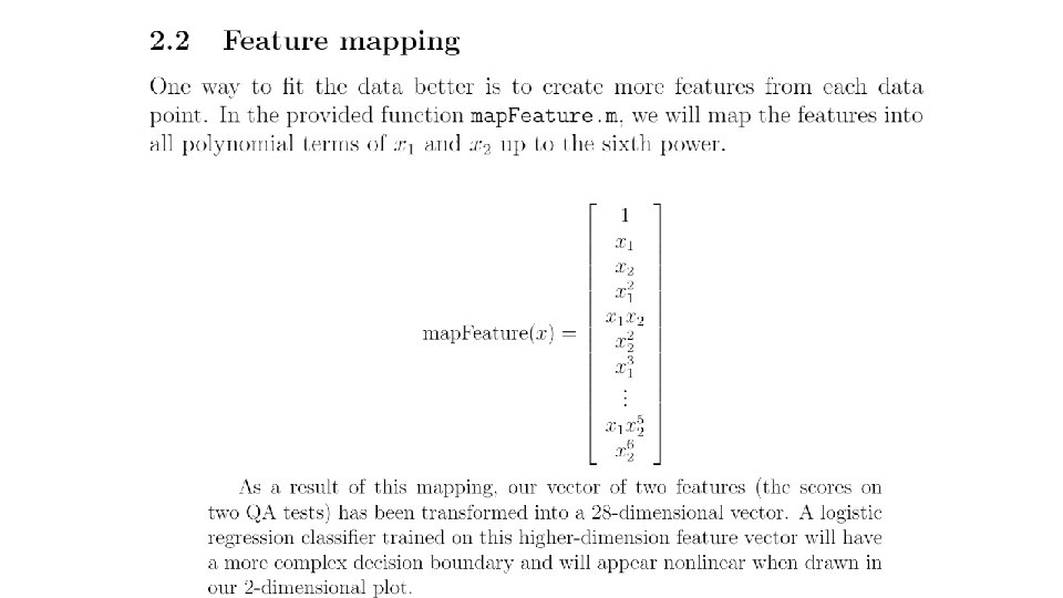
data = load('ex 2 data 2. txt'); X = data(: , [1, 2]); y = data(: , 3); X = map. Feature(X(: , 1), X(: , 2)); % size(X) = m, 28 initial_theta = zeros(size(X, 2), 1); % Set regularization parameter lambda to 1 lambda = 1; [cost, grad] = cost. Function. Reg(initial_theta, X, y, lambda); function out = map. Feature(X 1, X 2) degree = 6; out = ones(size(X 1(: , 1))); % size(out) = m, 1 for i = 1: degree for j = 0: i out(: , end+1) = (X 1. ^(i-j)). *(X 2. ^j); end %size(out) =m, 28 end
Regularized linear regression function [J, grad] = cost. Function. Reg(theta, X, y, lambda) m = length(y); % number of training examples J = 0; grad = zeros(size(theta)); h = sigmoid(X * theta); J = (1 / 2* m) * (-y' * log(h) - (1 - y') * log(1 - h)) +. . . (lambda/2*m)* (theta’ * theta – theta(1)^2 ;