Machine Learning Machine learning explores the study and



- Slides: 60

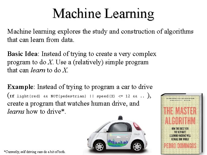
Machine Learning Machine learning explores the study and construction of algorithms that can learn from data. Basic Idea: Instead of trying to create a very complex program to do X. Use a (relatively) simple program that can learn to do X. Example: Instead of trying to program a car to drive (If light(red) && NOT(pedestrian) || speed(X) <= 12 &&. . ), create a program that watches human drive, and learns how to drive*. *Currently, self driving cars do a bit of both.

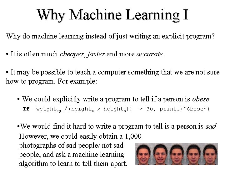
Why Machine Learning I Why do machine learning instead of just writing an explicit program? • It is often much cheaper, faster and more accurate. • It may be possible to teach a computer something that we are not sure how to program. For example: • We could explicitly write a program to tell if a person is obese If (weightkg /(heightm heightm)) > 30, printf(“Obese”) • We would find it hard to write a program to tell is a person is sad However, we could easily obtain a 1, 000 photographs of sad people/ not sad people, and ask a machine learning algorithm to learn to tell them apart.

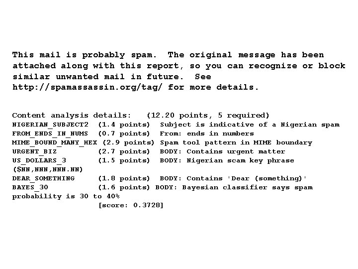
Why Machine Learning II Sometimes we need to relearn things at a speed that a human could not keep up with, if she had to keep rewriting code. • Imagine you wrote a spam classifier If observed(‘Nigeria’, ’$$$$’) || IP == 1. 160. 10. 240 || … • The moment you deployed this algorithm, the hackers could defeat it. • They could misspell keywords N 1 geria, Nig@ria • They could change their IP • Etc • What is needed here is an algorithm that relearns what spam is, every minute of the day, forever.

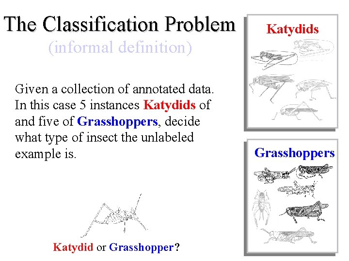
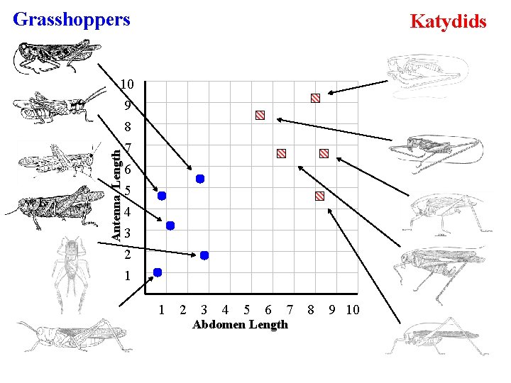
The Classification Problem Katydids (informal definition) Given a collection of annotated data. In this case 5 instances Katydids of and five of Grasshoppers, decide what type of insect the unlabeled example is. Katydid or Grasshopper? Grasshoppers

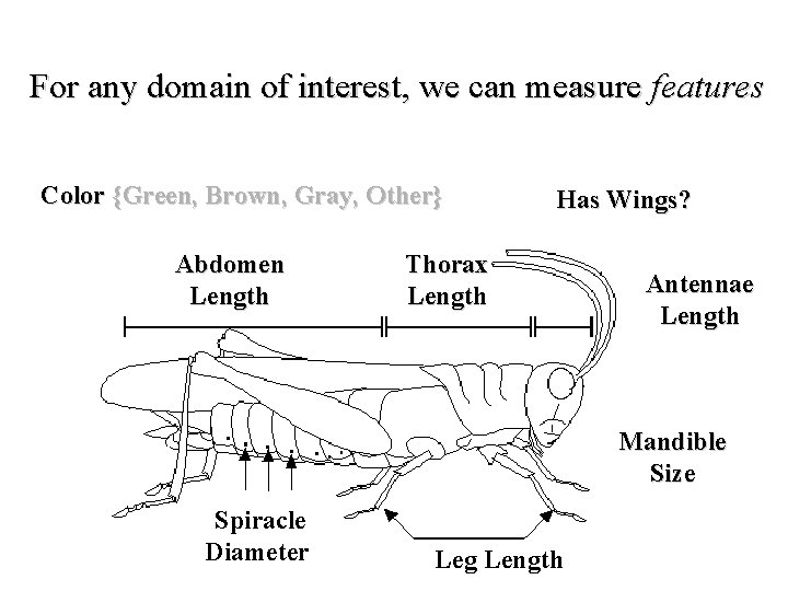
For any domain of interest, we can measure features Color {Green, Brown, Gray, Other} Abdomen Length Has Wings? Thorax Length Antennae Length Mandible Size Spiracle Diameter Leg Length

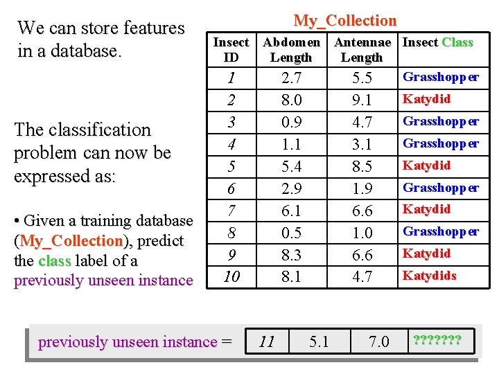
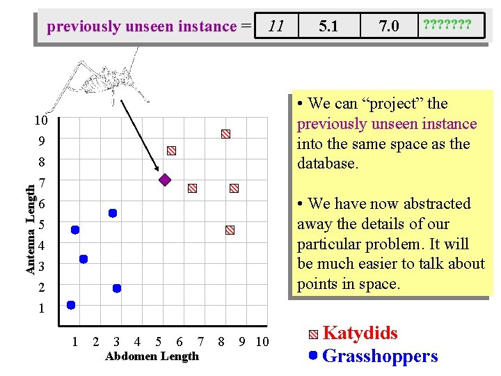
We can store features in a database. The classification problem can now be expressed as: • Given a training database (My_Collection), predict the class label of a previously unseen instance My_Collection Insect Abdomen Antennae Insect Class ID Length Grasshopper 1 2. 7 5. 5 2 3 4 5 6 7 8 9 10 previously unseen instance = 8. 0 0. 9 1. 1 5. 4 2. 9 6. 1 0. 5 8. 3 8. 1 11 9. 1 4. 7 3. 1 8. 5 1. 9 6. 6 1. 0 6. 6 4. 7 5. 1 7. 0 Katydid Grasshopper Katydids ? ? ? ?

Grasshoppers Katydids Antenna Length 10 9 8 7 6 5 4 3 2 1 1 2 3 4 5 6 7 Abdomen Length 8 9 10

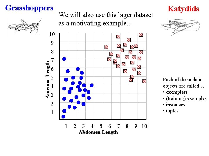
Grasshoppers We will also use this lager dataset as a motivating example… Katydids Antenna Length 10 9 8 7 6 5 Each of these data objects are called… • exemplars • (training) examples • instances • tuples 4 3 2 1 1 2 3 4 5 6 7 Abdomen Length 8 9 10

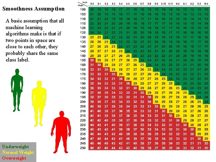
Smoothness Assumption A basic assumption that all machine learning algorithms make is that if two points in space are close to each other, they probably share the same class label. Underweight Normal Weight Overweight

We will return to the previous slide in two minutes. In the meantime, we are going to play a quick game. I am going to show you some classification problems which were shown to pigeons! Let us see if you are as smart as a pigeon!

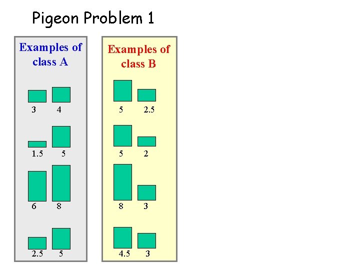
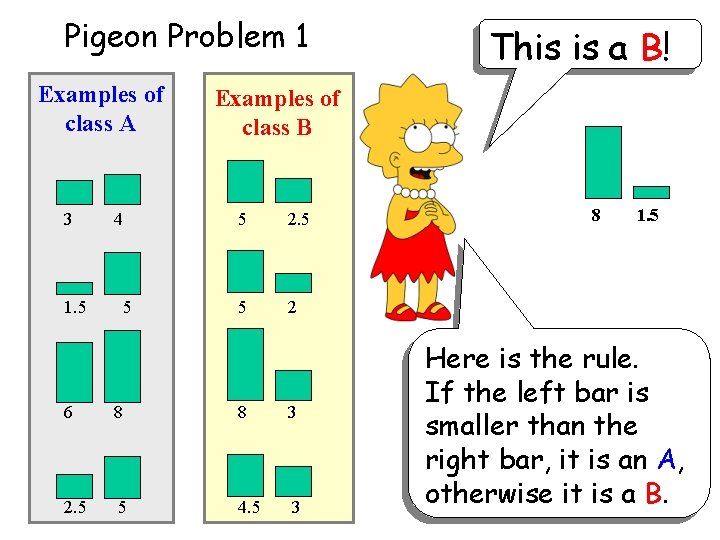
Pigeon Problem 1 Examples of class A Examples of class B 3 4 5 2. 5 1. 5 5 5 2 6 8 8 3 2. 5 5 4. 5 3

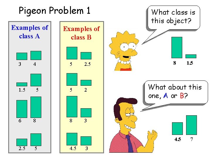
Pigeon Problem 1 Examples of class A Examples of class B 3 4 5 2. 5 1. 5 5 5 2 6 8 8 3 What class is this object? 8 What about this one, A or B? 4. 5 2. 5 5 4. 5 3 1. 5 7

Pigeon Problem 1 Examples of class A This is a B! Examples of class B 3 4 5 2. 5 1. 5 5 5 2 6 8 8 3 2. 5 5 4. 5 3 8 1. 5 Here is the rule. If the left bar is smaller than the right bar, it is an A, otherwise it is a B.

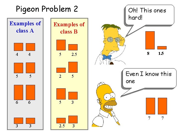
Pigeon Problem 2 Examples of class A Examples of class B 4 4 5 2. 5 5 5 2 5 6 6 5 3 Oh! This ones hard! 8 Even I know this one 7 3 3 2. 5 3 1. 5 7

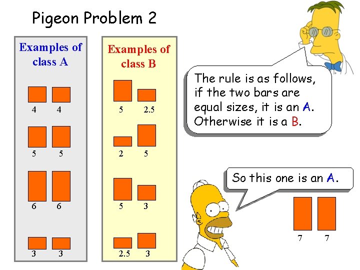
Pigeon Problem 2 Examples of class A Examples of class B 4 4 5 2. 5 5 5 2 5 The rule is as follows, if the two bars are equal sizes, it is an A. Otherwise it is a B. So this one is an A. 6 6 5 3 7 3 3 2. 5 3 7

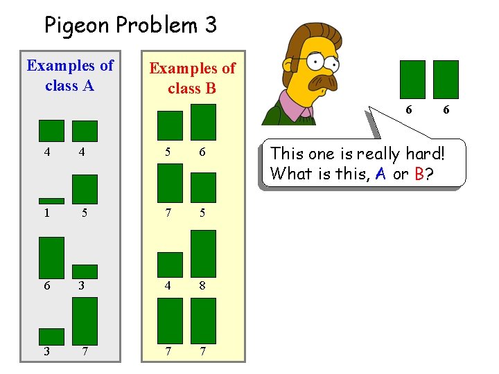
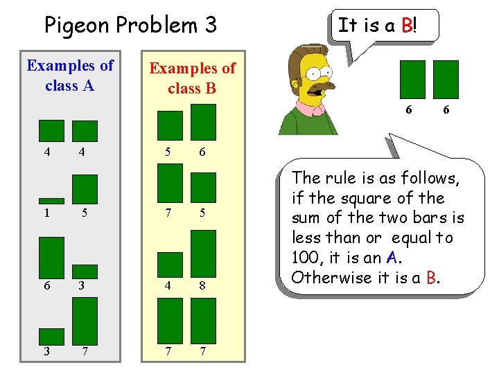
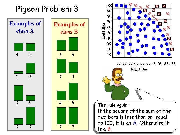
Pigeon Problem 3 Examples of class A Examples of class B 6 4 4 5 6 1 5 7 5 6 3 4 8 3 7 7 7 6 This one is really hard! What is this, A or B?

Pigeon Problem 3 Examples of class A It is a B! Examples of class B 6 4 4 6 5 6 1 5 7 5 6 3 4 8 3 7 7 7 The rule is as follows, if the square of the sum of the two bars is less than or equal to 100, it is an A. Otherwise it is a B.

Why did we spend so much time with this game? Because we wanted to show that almost all classification problems have a geometric interpretation, check out the next 3 slides…

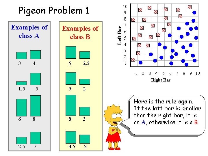
Examples of class A 3 4 Examples of class B 5 2. 5 Left Bar Pigeon Problem 1 10 9 8 7 6 5 4 3 2 1 1 2 3 4 5 6 7 8 9 10 Right Bar 1. 5 5 5 2 6 8 8 3 2. 5 5 4. 5 3 Here is the rule again. If the left bar is smaller than the right bar, it is an A, otherwise it is a B.

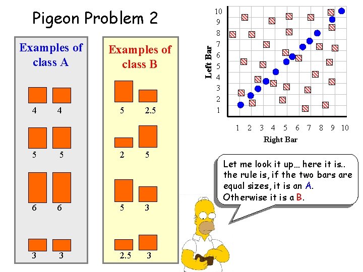
Examples of class A 4 4 Examples of class B 5 2. 5 Left Bar Pigeon Problem 2 10 9 8 7 6 5 4 3 2 1 1 2 3 4 5 6 7 8 9 10 Right Bar 5 5 2 5 6 6 5 3 3 3 2. 5 3 Let me look it up… here it is. . the rule is, if the two bars are equal sizes, it is an A. Otherwise it is a B.

Examples of class A 4 4 Examples of class B 5 6 Left Bar Pigeon Problem 3 100 90 80 70 60 50 40 30 20 10 10 20 30 40 50 60 70 80 90 100 Right Bar 1 5 7 5 6 3 4 8 3 7 7 7 The rule again: if the square of the sum of the two bars is less than or equal to 100, it is an A. Otherwise it is a B.

Grasshoppers Katydids Antenna Length 10 9 8 7 6 5 4 3 2 1 1 2 3 4 5 6 7 Abdomen Length 8 9 10

previously unseen instance = 11 7. 0 ? ? ? ? • We can “project” the previously unseen instance into the same space as the database. 10 Antenna Length 5. 1 9 8 7 • We have now abstracted away the details of our particular problem. It will be much easier to talk about points in space. 6 5 4 3 2 1 1 2 3 4 5 6 7 Abdomen Length 8 9 10 Katydids Grasshoppers

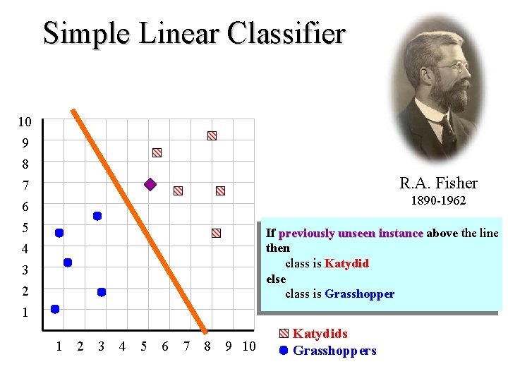
Simple Linear Classifier 10 9 8 7 R. A. Fisher 1890 -1962 6 5 4 3 2 1 If previously unseen instance above the line then class is Katydid else class is Grasshopper 1 2 3 4 5 6 7 8 9 10 Katydids Grasshoppers

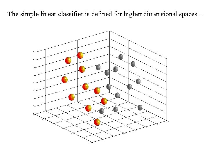
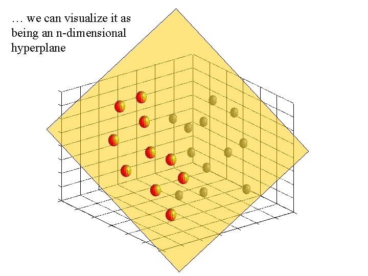
The simple linear classifier is defined for higher dimensional spaces…

… we can visualize it as being an n-dimensional hyperplane

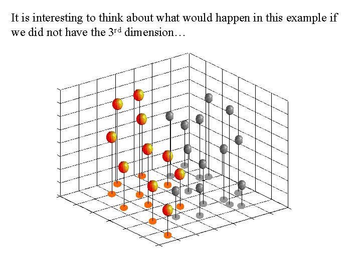
It is interesting to think about what would happen in this example if we did not have the 3 rd dimension…

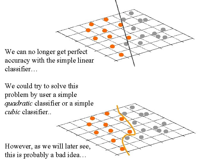
We can no longer get perfect accuracy with the simple linear classifier… We could try to solve this problem by user a simple quadratic classifier or a simple cubic classifier. . However, as we will later see, this is probably a bad idea…

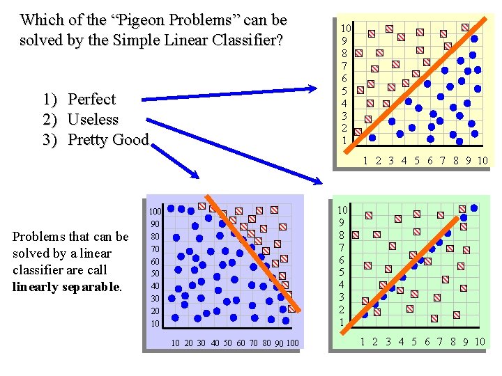
Which of the “Pigeon Problems” can be solved by the Simple Linear Classifier? 1) 2) 3) Perfect Useless Pretty Good 10 9 8 7 6 5 4 3 2 1 1 2 3 4 5 6 7 8 9 10 Problems that can be solved by a linear classifier are call linearly separable. 10 9 8 7 6 5 4 3 2 1 100 90 80 70 60 50 40 30 20 10 10 20 30 40 50 60 70 80 90 100 1 2 3 4 5 6 7 8 9 10

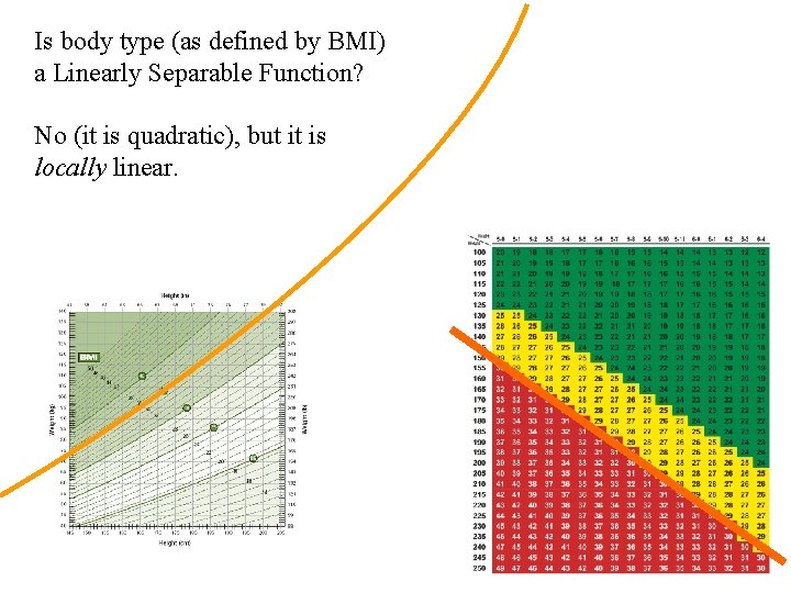
Is body type (as defined by BMI) a Linearly Separable Function? No (it is quadratic), but it is locally linear.

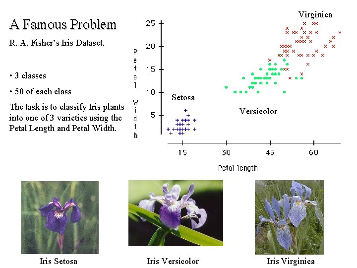
Virginica A Famous Problem R. A. Fisher’s Iris Dataset. • 3 classes • 50 of each class The task is to classify Iris plants into one of 3 varieties using the Petal Length and Petal Width. Iris Setosa Versicolor Iris Virginica

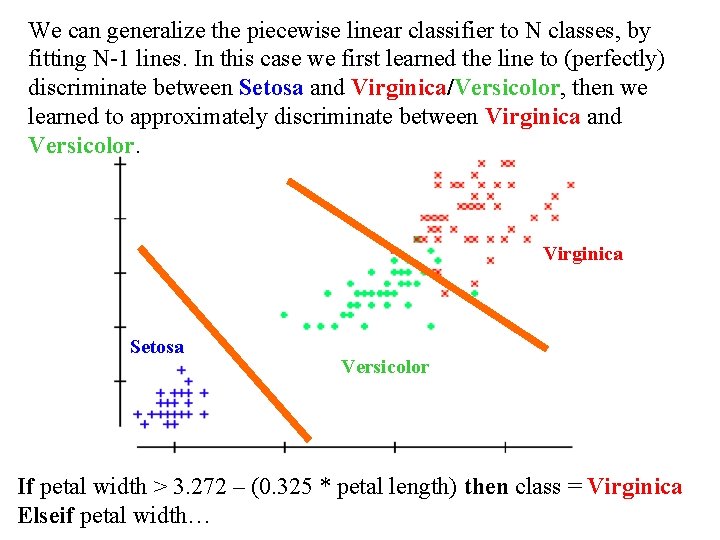
We can generalize the piecewise linear classifier to N classes, by fitting N-1 lines. In this case we first learned the line to (perfectly) discriminate between Setosa and Virginica/Versicolor, then we learned to approximately discriminate between Virginica and Versicolor. Virginica Setosa Versicolor If petal width > 3. 272 – (0. 325 * petal length) then class = Virginica Elseif petal width…

We have now seen one classification algorithm, and we are about to see more. How should we compare them? • Predictive accuracy • Speed and scalability – time to construct the model – time to use the model – efficiency in disk-resident databases • Robustness – handling noise, missing values and irrelevant features, streaming data • Interpretability: – understanding and insight provided by the model

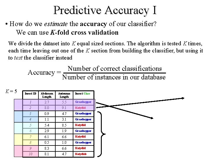
Predictive Accuracy I • How do we estimate the accuracy of our classifier? We can use K-fold cross validation We divide the dataset into K equal sized sections. The algorithm is tested K times, each time leaving out one of the K section from building the classifier, but using it to test the classifier instead Number of correct classifications Accuracy = Number of instances in our database K = 5 Insect ID Abdomen Length Antennae Length Insect Class 1 2. 7 5. 5 Grasshopper 2 8. 0 9. 1 Katydid 3 0. 9 4. 7 Grasshopper 4 1. 1 3. 1 Grasshopper 5 5. 4 8. 5 Katydid 6 2. 9 1. 9 Grasshopper 7 6. 1 6. 6 Katydid 8 0. 5 1. 0 Grasshopper 9 8. 3 6. 6 Katydid 10 8. 1 4. 7 Katydids

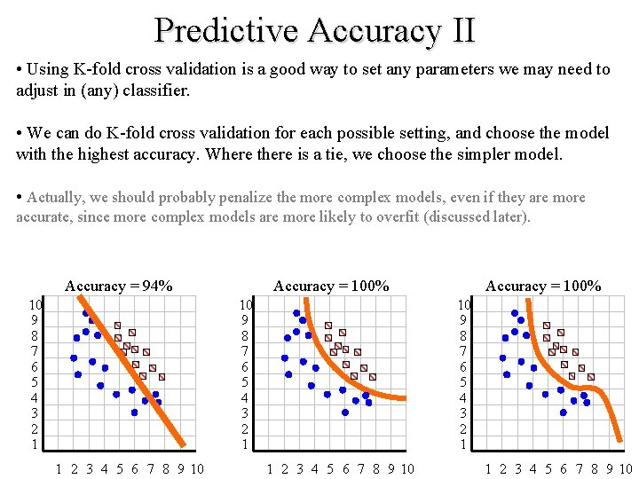
Predictive Accuracy II • Using K-fold cross validation is a good way to set any parameters we may need to adjust in (any) classifier. • We can do K-fold cross validation for each possible setting, and choose the model with the highest accuracy. Where there is a tie, we choose the simpler model. • Actually, we should probably penalize the more complex models, even if they are more accurate, since more complex models are more likely to overfit (discussed later). Accuracy = 94% 10 9 8 7 6 5 4 3 2 1 Accuracy = 100% 10 9 8 7 6 5 4 3 2 1 1 2 3 4 5 6 7 8 9 10

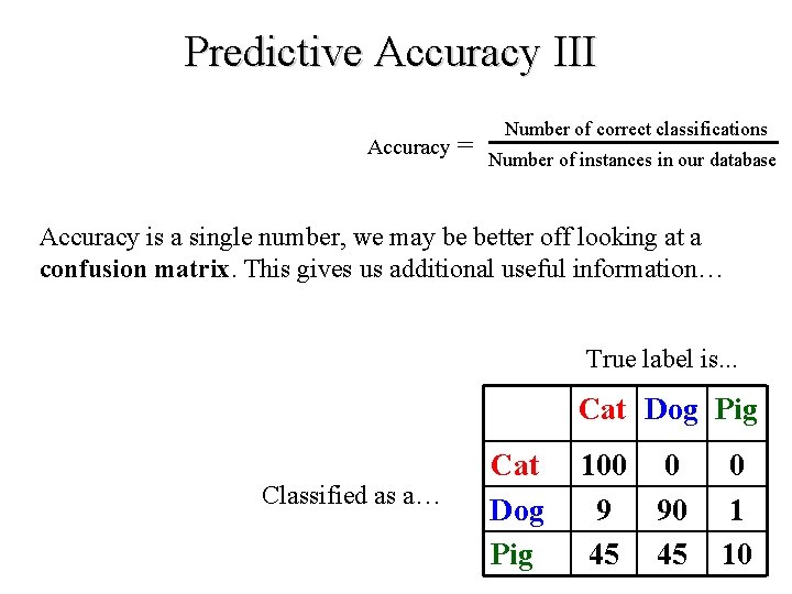
Predictive Accuracy III Accuracy = Number of correct classifications Number of instances in our database Accuracy is a single number, we may be better off looking at a confusion matrix. This gives us additional useful information… True label is. . . Cat Dog Pig Classified as a… Cat Dog Pig 100 0 9 90 45 45 0 1 10

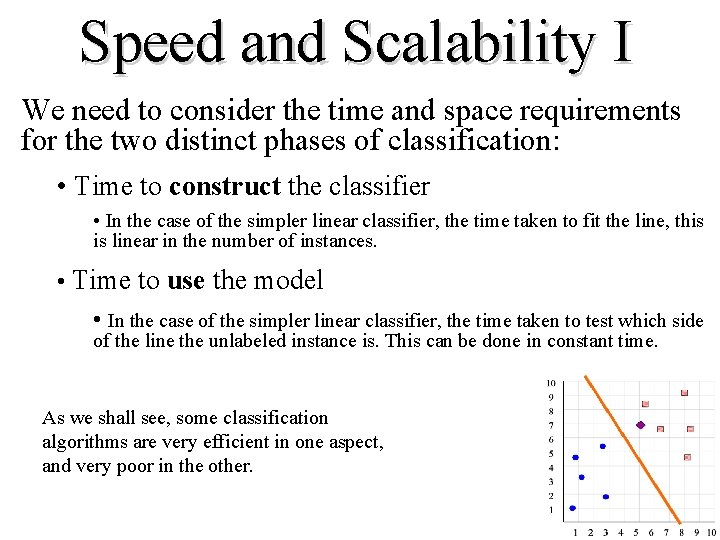
Speed and Scalability I We need to consider the time and space requirements for the two distinct phases of classification: • Time to construct the classifier • In the case of the simpler linear classifier, the time taken to fit the line, this is linear in the number of instances. • Time to use the model • In the case of the simpler linear classifier, the time taken to test which side of the line the unlabeled instance is. This can be done in constant time. As we shall see, some classification algorithms are very efficient in one aspect, and very poor in the other.

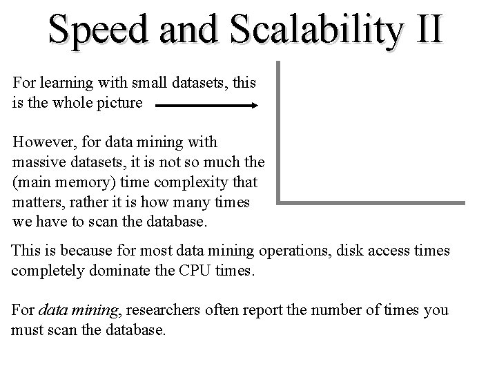
Speed and Scalability II For learning with small datasets, this is the whole picture However, for data mining with massive datasets, it is not so much the (main memory) time complexity that matters, rather it is how many times we have to scan the database. This is because for most data mining operations, disk access times completely dominate the CPU times. For data mining, researchers often report the number of times you must scan the database.

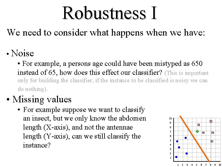
Robustness I We need to consider what happens when we have: • Noise • For example, a persons age could have been mistyped as 650 instead of 65, how does this effect our classifier? (This is important only for building the classifier, if the instance to be classified is noisy we can do nothing). • Missing values • For example suppose we want to classify an insect, but we only know the abdomen length (X-axis), and not the antennae length (Y-axis), can we still classify the instance? 10 9 8 7 6 5 4 3 2 1 1 2 3 4 5 6 7 8 9 10

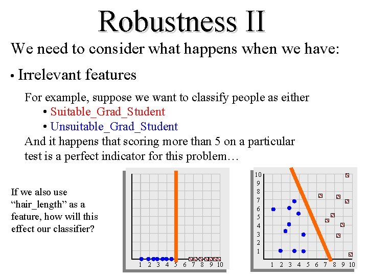
Robustness II We need to consider what happens when we have: • Irrelevant features For example, suppose we want to classify people as either • Suitable_Grad_Student • Unsuitable_Grad_Student And it happens that scoring more than 5 on a particular test is a perfect indicator for this problem… 10 9 8 7 6 5 4 3 2 1 If we also use “hair_length” as a feature, how will this effect our classifier? 1 2 3 4 5 6 7 8 9 10

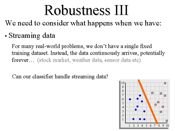
Robustness III We need to consider what happens when we have: • Streaming data For many real-world problems, we don’t have a single fixed training dataset. Instead, the data continuously arrives, potentially forever… (stock market, weather data, sensor data etc) Can our classifier handle streaming data? 10 9 8 7 6 5 4 3 2 1 1 2 3 4 5 6 7 8 9 10

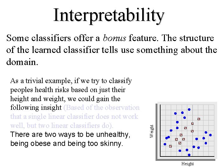
Interpretability Weight As a trivial example, if we try to classify peoples health risks based on just their height and weight, we could gain the following insight (Based of the observation that a single linear classifier does not work well, but two linear classifiers do). There are two ways to be unhealthy, being obese and being too skinny. Some classifiers offer a bonus feature. The structure of the learned classifier tells use something about the domain. Height

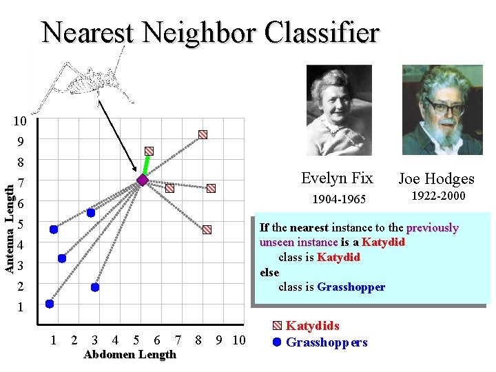
Nearest Neighbor Classifier Antenna Length 10 9 8 7 6 5 4 3 2 1 Evelyn Fix Joe Hodges 1904 -1965 1922 -2000 If the nearest instance to the previously unseen instance is unseen instance a Katydid class is Katydid else class is Grasshopper 1 2 3 4 5 6 7 Abdomen Length 8 9 10 Katydids Grasshoppers

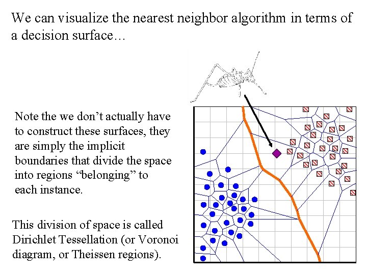
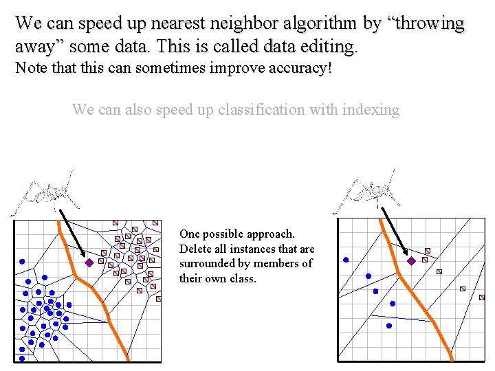
We can visualize the nearest neighbor algorithm in terms of a decision surface… Note the we don’t actually have to construct these surfaces, they are simply the implicit boundaries that divide the space into regions “belonging” to each instance. This division of space is called Dirichlet Tessellation (or Voronoi diagram, or Theissen regions).

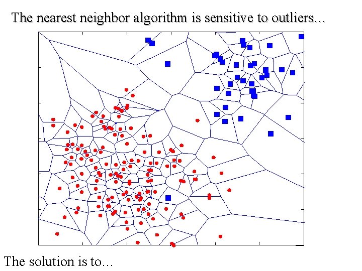
The nearest neighbor algorithm is sensitive to outliers… The solution is to…

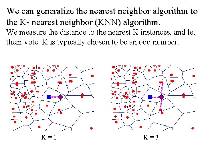
We can generalize the nearest neighbor algorithm to the K- nearest neighbor (KNN) algorithm. We measure the distance to the nearest K instances, and let them vote. K is typically chosen to be an odd number. K = 1 K = 3

Breadfruit (Artocarpus altilis) Hawaii 2015

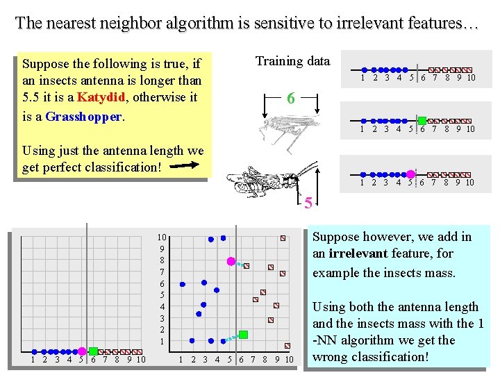
The nearest neighbor algorithm is sensitive to irrelevant features… Suppose the following is true, if an insects antenna is longer than 5. 5 it is a Katydid, otherwise it is a Grasshopper. Training data 1 2 3 4 5 6 7 8 9 10 6 1 2 3 4 5 6 7 8 9 10 Using just the antenna length we get perfect classification! 1 2 3 4 5 6 7 8 9 10 5 Suppose however, we add in an irrelevant feature, for example the insects mass. 10 9 8 7 6 5 4 3 2 1 1 2 3 4 5 6 7 8 9 10 Using both the antenna length and the insects mass with the 1 -NN algorithm we get the wrong classification!

How do we mitigate the nearest neighbor algorithms sensitivity to irrelevant features? • Use more training instances • Ask an expert what features are relevant to the task • Use statistical tests to try to determine which features are useful • Search over feature subsets (in the next slide we will see why this is hard)

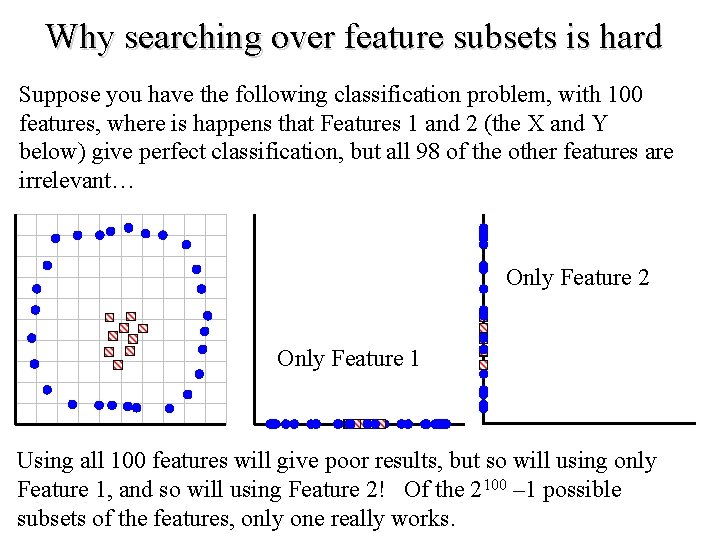
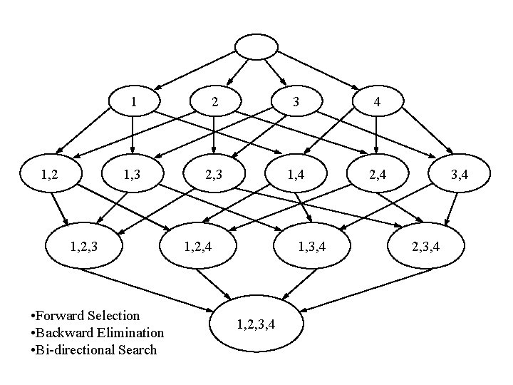
Why searching over feature subsets is hard Suppose you have the following classification problem, with 100 features, where is happens that Features 1 and 2 (the X and Y below) give perfect classification, but all 98 of the other features are irrelevant… Only Feature 2 Only Feature 1 Using all 100 features will give poor results, but so will using only Feature 1, and so will using Feature 2! Of the 2100 – 1 possible subsets of the features, only one really works.

1, 2 1 2 3 4 1, 3 2, 3 1, 4 2, 4 1, 2, 3 • Forward Selection • Backward Elimination • Bi-directional Search 1, 2, 4 1, 3, 4 1, 2, 3, 4

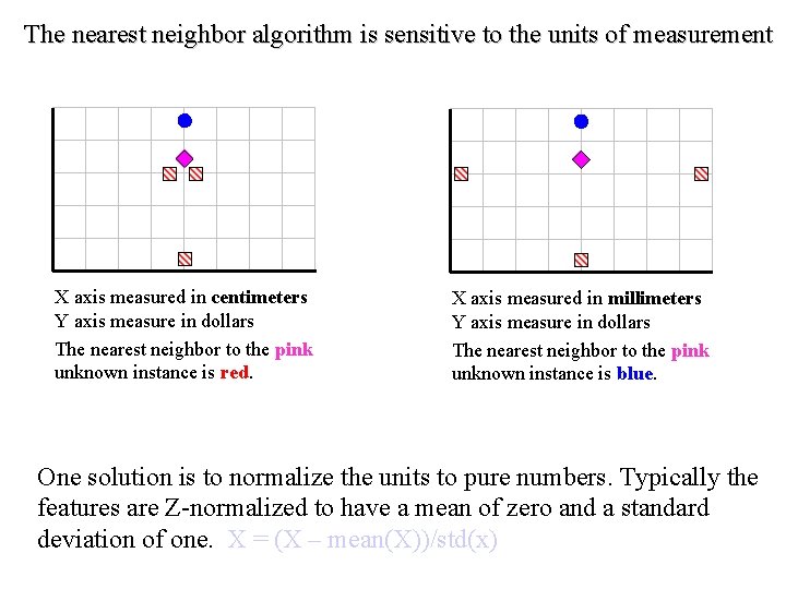
The nearest neighbor algorithm is sensitive to the units of measurement X axis measured in centimeters Y axis measure in dollars The nearest neighbor to the pink unknown instance is red. X axis measured in millimeters Y axis measure in dollars The nearest neighbor to the pink unknown instance is blue. One solution is to normalize the units to pure numbers. Typically the features are Z-normalized to have a mean of zero and a standard deviation of one. X = (X – mean(X))/std(x)

We can speed up nearest neighbor algorithm by “throwing away” some data. This is called data editing. Note that this can sometimes improve accuracy! We can also speed up classification with indexing One possible approach. Delete all instances that are surrounded by members of their own class.

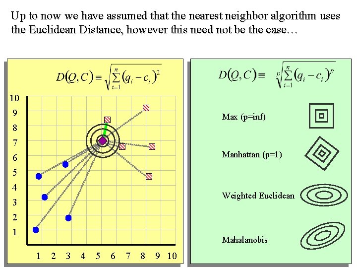
Up to now we have assumed that the nearest neighbor algorithm uses the Euclidean Distance, however this need not be the case… 10 9 8 7 6 5 4 3 2 1 Max (p=inf) Manhattan (p=1) Weighted Euclidean Mahalanobis 1 2 3 4 5 6 7 8 9 10

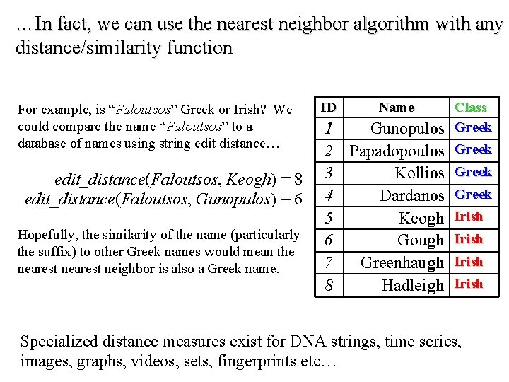
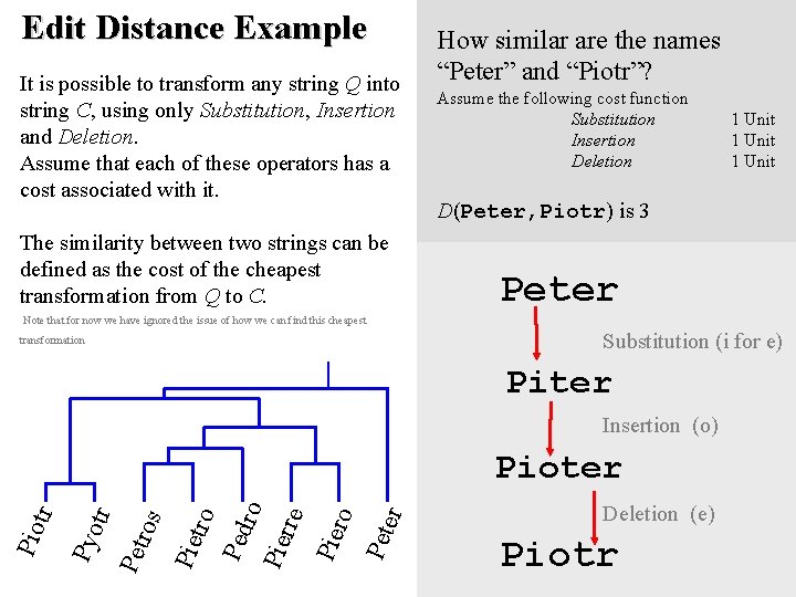
…In fact, we can use the nearest neighbor algorithm with any distance/similarity function For example, is “Faloutsos” Greek or Irish? We could compare the name “Faloutsos” to a database of names using string edit distance… edit_distance(Faloutsos, Keogh) = 8 edit_distance(Faloutsos, Gunopulos) = 6 Hopefully, the similarity of the name (particularly the suffix) to other Greek names would mean the nearest neighbor is also a Greek name. ID Name Class Greek 1 Gunopulos 2 Papadopoulos Greek 3 Kollios Greek 4 Dardanos Greek 5 Keogh Irish 6 Gough Irish 7 Greenhaugh Irish 8 Hadleigh Irish Specialized distance measures exist for DNA strings, time series, images, graphs, videos, sets, fingerprints etc…

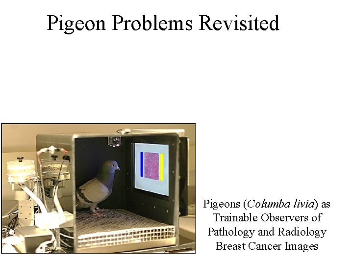
Pigeon Problems Revisited Pigeons (Columba livia) as Trainable Observers of Pathology and Radiology Breast Cancer Images

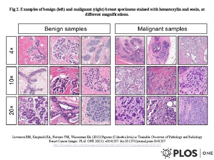
Fig 2. Examples of benign (left) and malignant (right) breast specimens stained with hematoxylin and eosin, at different magnifications. Levenson RM, Krupinski EA, Navarro VM, Wasserman EA (2015) Pigeons (Columba livia) as Trainable Observers of Pathology and Radiology Breast Cancer Images. PLo. S ONE 10(11): e 0141357. doi: 10. 1371/journal. pone. 0141357 http: //journals. plos. org/plosone/article? id=info: doi/10. 1371/journal. pone. 0141357

Dear SIR, I am Mr. John Coleman and my sister is Miss Rose Colemen, we are the children of late Chief Paul Colemen from Sierra Leone. I am writing you in absolute confidence primarily to seek your assistance to transfer our cash of twenty one Million Dollars ($21, 000. 00) now in the custody of a private Security trust firm in Europe the money is in trunk boxes deposited and declared as family valuables by my late father as a matter of fact the company does not know the content as money, although my father made them to under stand that the boxes belongs to his foreign partner. …

This mail is probably spam. The original message has been attached along with this report, so you can recognize or block similar unwanted mail in future. See http: //spamassassin. org/tag/ for more details. Content analysis details: (12. 20 points, 5 required) NIGERIAN_SUBJECT 2 (1. 4 points) Subject is indicative of a Nigerian spam FROM_ENDS_IN_NUMS (0. 7 points) From: ends in numbers MIME_BOUND_MANY_HEX (2. 9 points) Spam tool pattern in MIME boundary URGENT_BIZ (2. 7 points) BODY: Contains urgent matter US_DOLLARS_3 (1. 5 points) BODY: Nigerian scam key phrase ($NN, NNN. NN) DEAR_SOMETHING (1. 8 points) BODY: Contains 'Dear (something)' BAYES_30 (1. 6 points) BODY: Bayesian classifier says spam probability is 30 to 40% [score: 0. 3728]

Edit Distance Example It is possible to transform any string Q into string C, using only Substitution, Insertion and Deletion. Assume that each of these operators has a cost associated with it. The similarity between two strings can be defined as the cost of the cheapest transformation from Q to C. Note that for now we have ignored the issue of how we can find this cheapest transformation How similar are the names “Peter” and “Piotr”? Assume the following cost function Substitution Insertion Deletion D(Peter, Piotr) is 3 Peter Substitution (i for e) Piter Insertion (o) er Pet Ped ro Pie rre Pie ro tro Pie ros Pet tr Pyo tr Pioter Pio 1 Unit Deletion (e) Piotr