Part IB Descriptive Statistics Multivariate Statistics Focus Multiple

Part IB. Descriptive Statistics Multivariate Statistics (多變量統計) Focus: Multiple regression Spring 2007 1

Regression Analysis (迴歸分析) • Y = f(X): Y is a function of X • Regression analysis: a method of determining the specific function relating Y to X • Linear Regression (線性迴歸分析): a popular model in social science • A brief review offered here – Can see ppt files on the course website 2

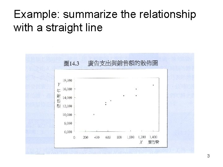
Example: summarize the relationship with a straight line 3

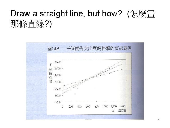
Draw a straight line, but how? (怎麼畫 那條直線? ) 4

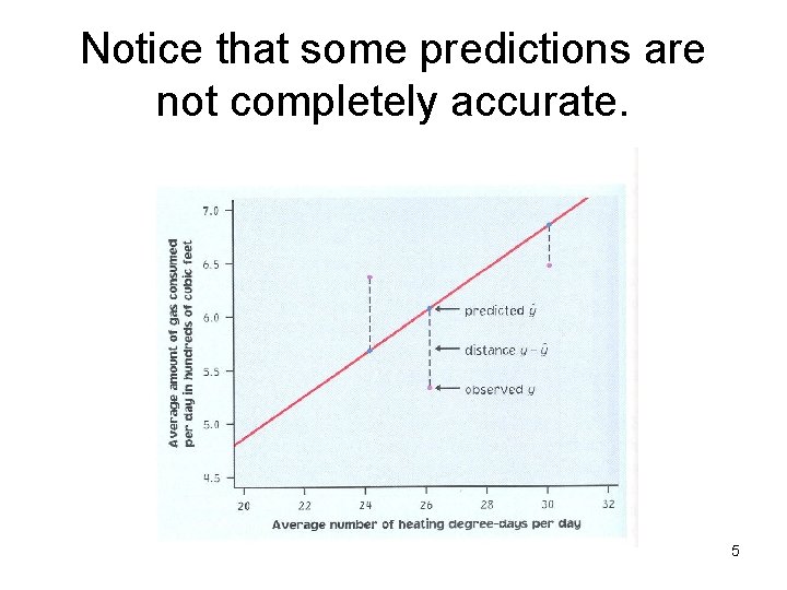
Notice that some predictions are not completely accurate. 5

How to draw the line? • Purpose: draw the regression line to give the most accurate predictions of y given x • Criteria for “accurate”: Sum of (observed y – predicted y)2 = sum of (prediction errors) 2 [觀察值與估計值之差的平方和] Called the sum of squared errors or sum of the squared residuals (SSE) 6

Ordinary Least Squares (OLS) Regression (普通最小平方法) • The regression line is drawn so as to minimize the sum of the squared vertical distances from the points to the line (讓SSE最小) • This line minimize squared predictive error • This line will pass through the middle of the point cloud (迴歸線從資料群中間穿過 )(think as a nice choice to describe the relationship) 7

To describe a regression line (equation): • Algebraically, line described by its intercept (截 距) and slope (斜率) • Notation: y = the dependent variable x = the independent variable y_hat = predicted y, based on the regression line β = slope of the regression line α= intercept of the regression line 8

The meaning of slope and intercept: • slope = change in (y_hat) for a 1 unit change in x (x一單位的改變導致y估計值 的變化) • intercept = value of (y_hat) when x is 0 • 解釋截距與斜率時要注意到x and y的單 位 9

General equation of a regression line: (y_hat) = α +βx where α and β are chosen to minimize: sum of (observed y – predicted y)2 A formula for α and β which minimize this sum is programmed into statistical programs and calculators 10

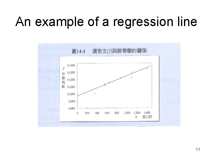
An example of a regression line 11

Fit: how much can regression explain? (迴歸能解釋y多少的變異？ ) • Look at the regression equation again: (y_hat) = α +βx y = α +βx + ε • Data = what we explain + what we don’t explain • Data = predicted + residual (資料有我們不能解釋的與可解釋的部分，即 能預估的與誤差的部分） 12

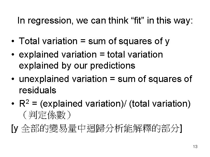
In regression, we can think “fit” in this way: • Total variation = sum of squares of y • explained variation = total variation explained by our predictions • unexplained variation = sum of squares of residuals • R 2 = (explained variation)/ (total variation) （判定係數） [y 全部的變易量中迴歸分析能解釋的部分] 13

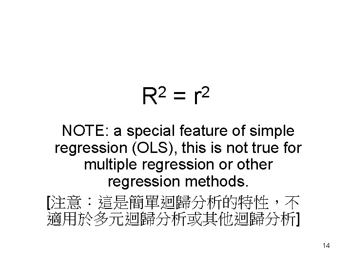
2 R = 2 r NOTE: a special feature of simple regression (OLS), this is not true for multiple regression or other regression methods. [注意：這是簡單迴歸分析的特性，不 適用於多元迴歸分析或其他迴歸分析] 14

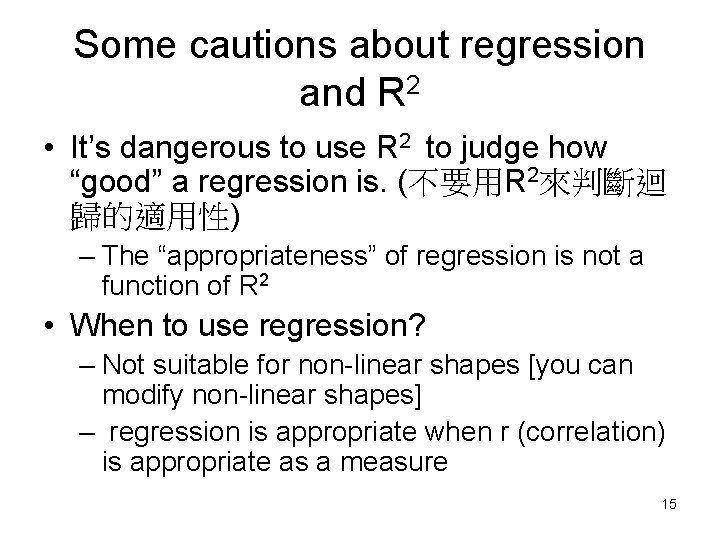
Some cautions about regression and R 2 • It’s dangerous to use R 2 to judge how “good” a regression is. (不要用R 2來判斷迴 歸的適用性) – The “appropriateness” of regression is not a function of R 2 • When to use regression? – Not suitable for non-linear shapes [you can modify non-linear shapes] – regression is appropriate when r (correlation) is appropriate as a measure 15

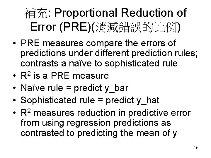
補充: Proportional Reduction of Error (PRE)(消減錯誤的比例) • PRE measures compare the errors of predictions under different prediction rules; contrasts a naïve to sophisticated rule • R 2 is a PRE measure • Naïve rule = predict y_bar • Sophisticated rule = predict y_hat • R 2 measures reduction in predictive error from using regression predictions as contrasted to predicting the mean of y 16

Cautions about correlation and regression: • Extrapolation is not appropriate • Regression: pay attention to lurking or omitted variables – Lurking (omitted) variables: having influence on the relationship between two variables but is not included among the variables studied – A problem in establishing causation • Association does not imply causation. – Association alone: weak evidence about causation – Experiments with random assignment are the best way to establish causation. 17

Inference for Simple Regression 18

Regression Equation of a regression line: (y_hat) = α +βx y = α +βx + ε y = dependent variable x = independent variable β = slope = predicted change in y with a one unit change in x α= intercept = predicted value of y when x is 0 y_hat = predicted value of dependent variable 19

21

The regression model (迴歸模型) • Note: the slope and intercept of the regression line are statistics (i. e. , from the sample data). • To do inference, we have to think of α and β as estimates of unknown parameters. 22

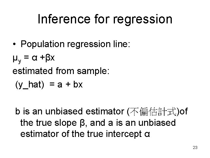
Inference for regression • Population regression line: μy = α +βx estimated from sample: (y_hat) = a + bx b is an unbiased estimator (不偏估計式)of the true slope β, and a is an unbiased estimator of the true intercept α 23

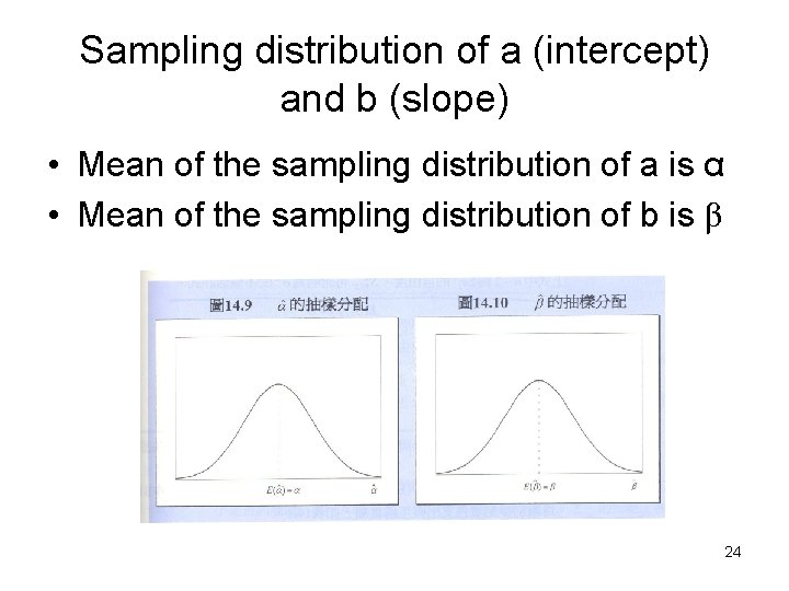
Sampling distribution of a (intercept) and b (slope) • Mean of the sampling distribution of a is α • Mean of the sampling distribution of b is β 24

Sampling distribution of a (intercept) and b (slope) • Mean of the sampling distribution of a is α • Mean of the sampling distribution of b is β • The standard error of a and b are related to the amount of spread about the regression line (σ) • Normal sampling distributions; with σ estimated use t-distribution for inference 25

The standard error of the least-squares line • Estimate σ (spread about the regression line using residuals from the regression) • recall that residual = (y –y_hat) • Estimate the population standard deviation about the regression line (σ) using the sample estimates 26

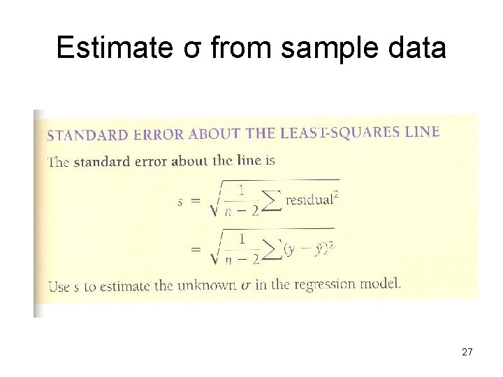
Estimate σ from sample data 27

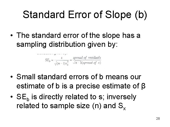
Standard Error of Slope (b) • The standard error of the slope has a sampling distribution given by: • Small standard errors of b means our estimate of b is a precise estimate of β • SEb is directly related to s; inversely related to sample size (n) and Sx 28

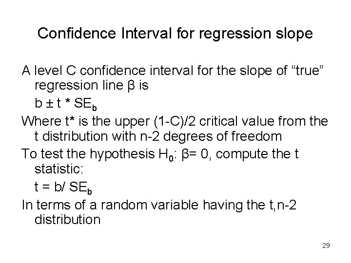
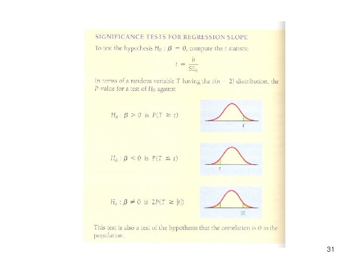
Confidence Interval for regression slope A level C confidence interval for the slope of “true” regression line β is b ± t * SEb Where t* is the upper (1 -C)/2 critical value from the t distribution with n-2 degrees of freedom To test the hypothesis H 0: β= 0, compute the t statistic: t = b/ SEb In terms of a random variable having the t, n-2 distribution 29

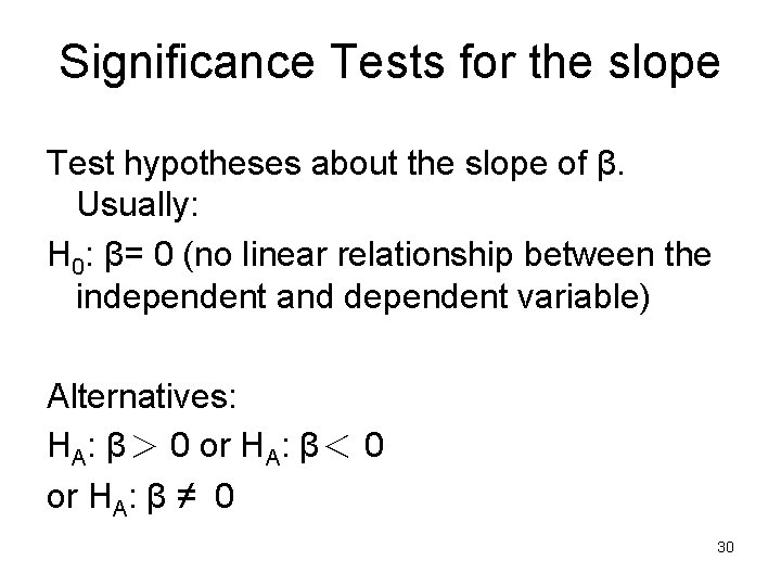
Significance Tests for the slope Test hypotheses about the slope of β. Usually: H 0: β= 0 (no linear relationship between the independent and dependent variable) Alternatives: HA: β＞ 0 or HA: β＜ 0 or HA: β ≠ 0 30

31

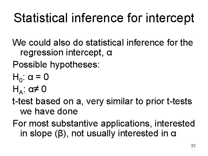
Statistical inference for intercept We could also do statistical inference for the regression intercept, α Possible hypotheses: H 0: α = 0 HA: α≠ 0 t-test based on a, very similar to prior t-tests we have done For most substantive applications, interested in slope (β), not usually interested in α 32

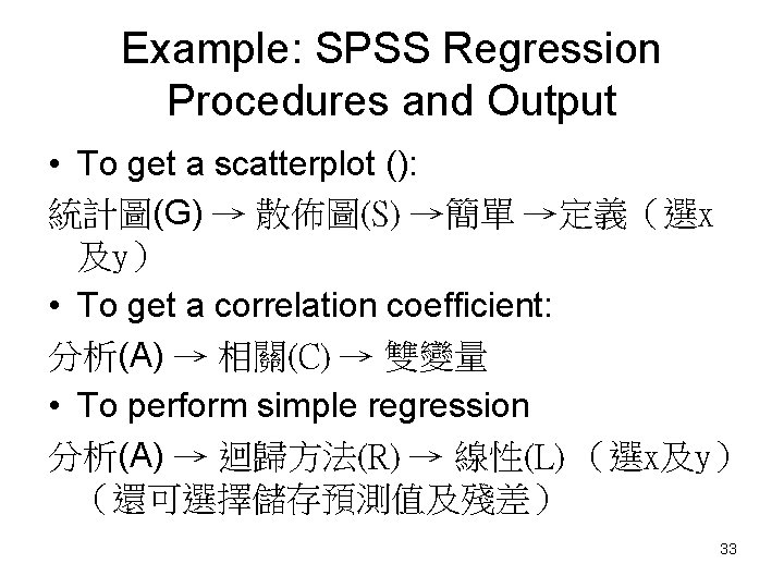
Example: SPSS Regression Procedures and Output • To get a scatterplot (): 統計圖(G) → 散佈圖(S) →簡單 →定義（選x 及y） • To get a correlation coefficient: 分析(A) → 相關(C) → 雙變量 • To perform simple regression 分析(A) → 迴歸方法(R) → 線性(L) （選x及y） （還可選擇儲存預測值及殘差） 33

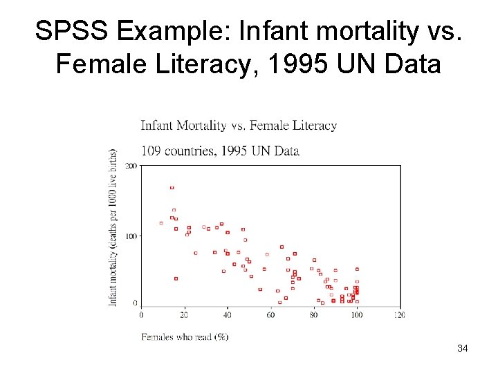
SPSS Example: Infant mortality vs. Female Literacy, 1995 UN Data 34

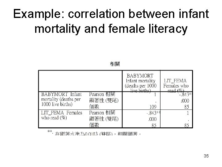
Example: correlation between infant mortality and female literacy 35

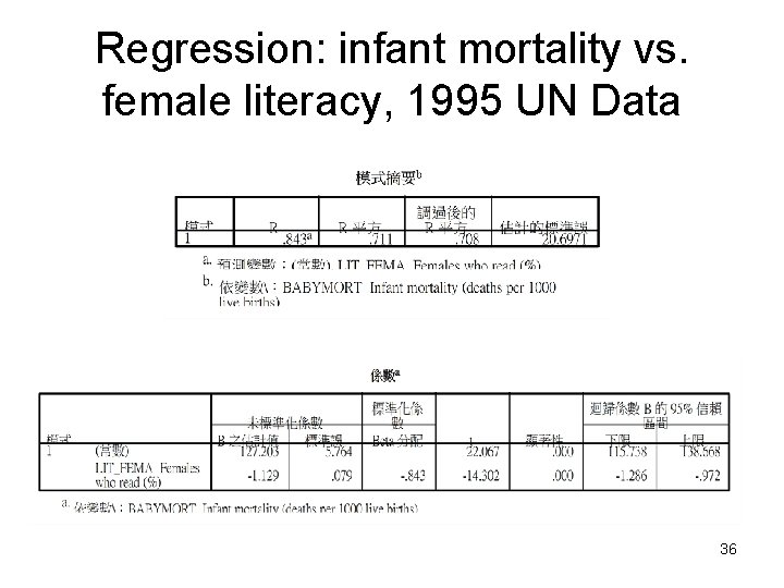
Regression: infant mortality vs. female literacy, 1995 UN Data 36

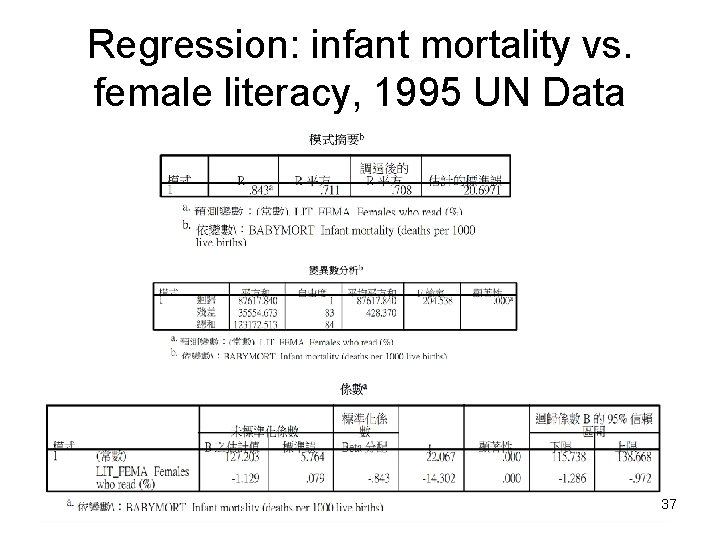
Regression: infant mortality vs. female literacy, 1995 UN Data 37