Machine Learning Makes it Predictive JMP Makes it

Machine Learning Makes it Predictive; JMP Makes it Explanatory

Abstract • Machine Learning is about creating predictive models. If the Target (aka. Response) is nominal, then a good model will maximize true positives and minimize false positives. This can provide information on dispositioning for instance. • Designed Experiments will use many of the same analysis algorithms but the focus is on causality and the appropriate recipe for success. JMP users may be more used to this paradigm so will often looking at models and ask “Why is the prediction so high? How do we improve it? What is important about the business? ” These questions are asking predictive models to become explanatory. The difference between predictive and root cause can be overlooked; yet we know correlation does not imply causation. The art of explaining data is getting lost in the push for advanced modeling techniques. • These questions can be hard to answer: restricted ranges on the variables, multicollinearity can make it very difficult to go from a predictive model to an explanatory model. Further, numeric summaries of models do not encourage subject matter experts to ask questions. The humble Profiler in JMP is a powerful tool in making models talk. • This presentation reminds us that, even for a data miner, it is the Profiler and Graph Builder that will make the difference.

Overview of Talk 1. Discussion of the issues and the purpose of modeling (predictive and explanatory) 2. Example demonstrating 1. Understanding the data. The usual EDA plus: Categories of Variables, Relevant time periods and process paths and data values. 2. Preparing the data for modeling 3. Modeling the data and machine learning models: variable selection using subject matter expertise and empirical information 4. Making the models explanatory: Profiler 3. Summary

Explanatory • Prediction is, given a new set of x’s, what will the response be • Models are More Explanatory (explanation) when it: • • Provides insight into why the response will be what it is Moves you toward root cause; helps you to understand the causal structure Provides engineering insights Challenges your understanding of the (work / business) process

What is Machine Learning Trying to gain information from stored data (by modeling) The functional form of the model can be hard to interpret Interpreting the functional form is fundamental to being explanatory There are reasons different modeling techniques might represent the process better than others • There are many modeling methods on the continuum from Classical Statistical methods to Machine Learning. • • • Bridging Prediction and Explanation is an issue in all models. We want something that we can interpret, and best represent the process. We want “new clues” to outcomes.

The Modeling Process Predictive Business Needs, Theories, Expectations, Predictions Available Data Exploratory Data Analysis Categories of Variables Nominal or continuous target? Segmentation Data Partition Variable Selection Data Modeling Model Selection Explanatory Model Application; Prediction Model Application; Explanation

Explanatory and Design of Experiments • Design of Experiments are naturally explanatory – why? • • Factors are manipulated according to a design matrix Defined confounding Randomization Balanced level settings This is why we’re having this discussion – we want to accomplish this with stored data. None of this is guaranteed with stored data (and machine learning)

Stored Data: Analysis Checklist 1. 2. 3. 4. 5. 6. Identify variables 1. Inputs 2. 3. Categories – e. g. , lines, product (nominal variables) Outputs 1. 2. 3. Controllable – willing to adjust Controllable – Unlikely to adjust Uncontrollable / noise Data Cleaning Sparklines – Plot Output and Inputs over time 1. 2. Have as many rows plotted as reasonable (use column switcher as well) Note extreme values – are they data issues (drop? ) or the most important data points Bivariate plots – Plot especially pairs of inputs (use column switcher) Variable clustering – in PCA platform Use modeling to focus on what matters.

Current_Between. Batch. Data. V 2. jmp Demonstration

Categories of Variables

Categories of Variables

Control Charting the Response over time Phase by Tank

Overlay Plot of the Response over time Color by Tank

“Spark Lines” – Plots over Time

Bivariate Plots

JMP Instructions for Bivariate Purit y

Missing Values in Controllable Variables

Principal Component Analysis (PCA) on Controllable and In-Process Variables

Cluster Variables Option in PCA Cluster Members 1 1 2 2 3 5 5 5 6 6 7 7 8 8 9 9 10 3 3 4 4 RSquare with 1 -RSquare Own Cluster Next Closest Ratio X 2_SP 0. 991 0. 027 0. 009 Additive 0. 991 0. 029 0. 009 Fan. Load 0. 738 0. 025 0. 269 X 4_Actual 0. 692 0. 04 0. 32 X 1_SP 0. 508 0. 162 0. 587 Dispersant 0. 163 0. 047 0. 878 Max. Temperature_ 0. 827 0. 013 0. 175 Top Max. Temperature 0. 682 0. 011 0. 321 Min 2 Avg. Feed. Rate 0. 294 0. 023 0. 723 C 0. 693 0. 075 0. 332 Ratio 0. 554 0. 027 0. 458 TAG_008 0. 458 0. 004 0. 544 TAG_012 0. 011 0. 002 0. 991 PRESSUREAt. T 3 TEMPAt. T 3 Feeder. B_Max MIXER_KW Add 2 X 3_SP A TAG_013 Feeder. A_Max C_Purity TAG_003 TAG_011 RSquare with 1 -RSquare Own Cluster Next Closest Ratio 0. 715 0. 026 0. 292 0. 678 0. 06 0. 343 0. 118 0. 003 0. 885 0. 606 0. 041 0. 411 0. 606 0. 081 0. 429 0. 528 0. 002 0. 473 0. 528 0. 005 0. 474 0. 517 0. 001 0. 483 0. 517 0. 004 0. 485 0. 514 0. 006 0. 489 0. 514 0. 034 0. 503 1 0. 002 0

Data to Model • Modeling assigns variation in the response to variation in the model’s inputs. • Modeling requires that there is variation • That data must come from a (relatively) stable process. Inconsistent data may be: • An attempt to model chaos • An average model that does not provide adequate operational specifics.

Why does JMP make it explanatory 1. Profiler 1. Desirability 2. Lots of ways to plot your data 1. i. e. , question what the model suggests 1. 2. 3. Bivariate plots Time series plots Distributions

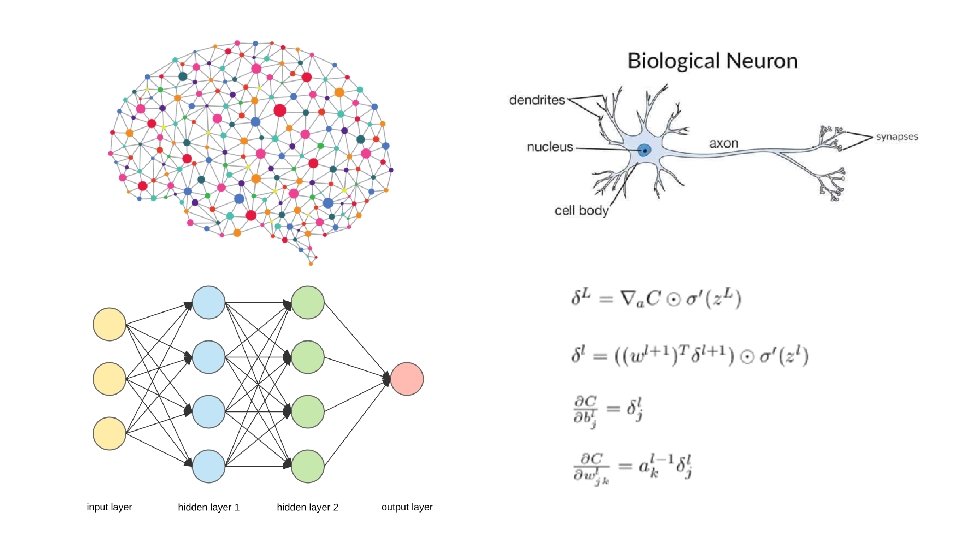
A Neural Network • Input comes into the brain and each level of neurons provide insight that gets passed on to the next level • In our artificial neural network, the “input” comes in the form of a training dataset in which a target variable has been identified that differentiates a response • Once trained (see the first bullet), it will try to classify new data based on what it thinks it’s experiencing throughout different units. • The output is compared to validation datasets that provide examples of what should be observed. • If they are the same, the neural net is validated. • If it’s incorrect, it uses back propagation to adjust its learning—going back through layers to recalibrate its perception of the process - This is deep learning, this is what makes a network intelligent.

Candidate Model

Yes Black Box No TBD 0. 95 0. 04 0. 01

Deep Learning Analytical Insights Older Learning Algorithms Amount of Data

JMP Profiler