Multivariate Linear Regression Chapter 8 1 Multivariate Analysis

Multivariate Linear Regression Chapter 8 1

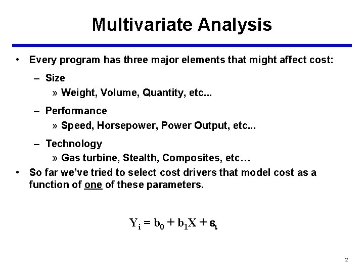
Multivariate Analysis • Every program has three major elements that might affect cost: – Size » Weight, Volume, Quantity, etc. . . – Performance » Speed, Horsepower, Power Output, etc. . . – Technology » Gas turbine, Stealth, Composites, etc… • So far we’ve tried to select cost drivers that model cost as a function of one of these parameters. Yi = b 0 + b 1 X + i 2

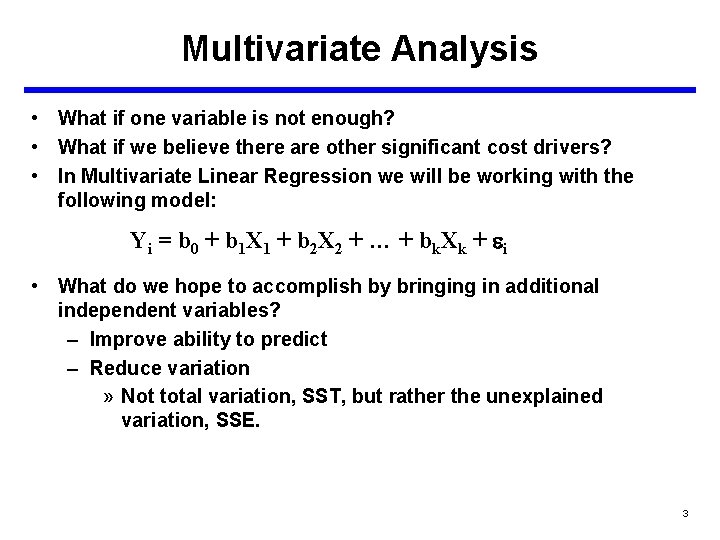
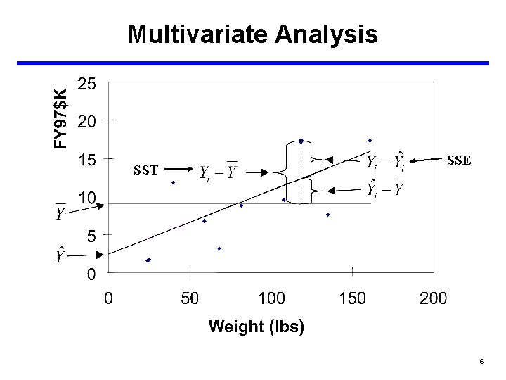
Multivariate Analysis • What if one variable is not enough? • What if we believe there are other significant cost drivers? • In Multivariate Linear Regression we will be working with the following model: Yi = b 0 + b 1 X 1 + b 2 X 2 + … + bk. Xk + i • What do we hope to accomplish by bringing in additional independent variables? – Improve ability to predict – Reduce variation » Not total variation, SST, but rather the unexplained variation, SSE. 3

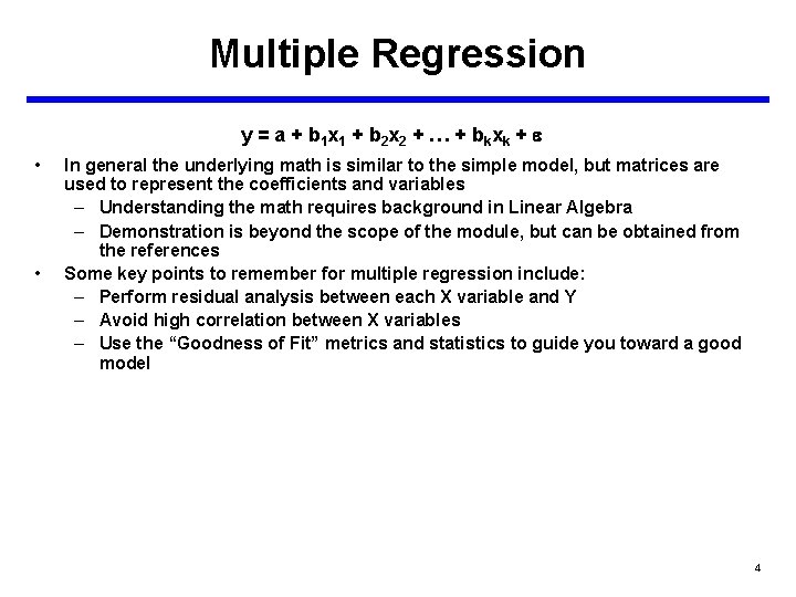
Multiple Regression y = a + b 1 x 1 + b 2 x 2 + … + b k xk + • • In general the underlying math is similar to the simple model, but matrices are used to represent the coefficients and variables – Understanding the math requires background in Linear Algebra – Demonstration is beyond the scope of the module, but can be obtained from the references Some key points to remember for multiple regression include: – Perform residual analysis between each X variable and Y – Avoid high correlation between X variables – Use the “Goodness of Fit” metrics and statistics to guide you toward a good model 4

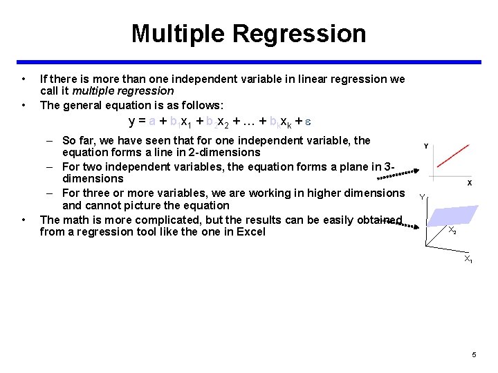
Multiple Regression • • If there is more than one independent variable in linear regression we call it multiple regression The general equation is as follows: y = a + b 1 x 1 + b 2 x 2 + … + bkxk + e • – So far, we have seen that for one independent variable, the equation forms a line in 2 -dimensions – For two independent variables, the equation forms a plane in 3 dimensions – For three or more variables, we are working in higher dimensions and cannot picture the equation The math is more complicated, but the results can be easily obtained from a regression tool like the one in Excel Y X 2 X 1 5

Multivariate Analysis SST SSE 6

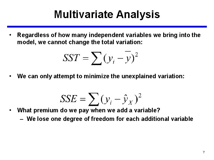
Multivariate Analysis • Regardless of how many independent variables we bring into the model, we cannot change the total variation: • We can only attempt to minimize the unexplained variation: • What premium do we pay when we add a variable? – We lose one degree of freedom for each additional variable 7

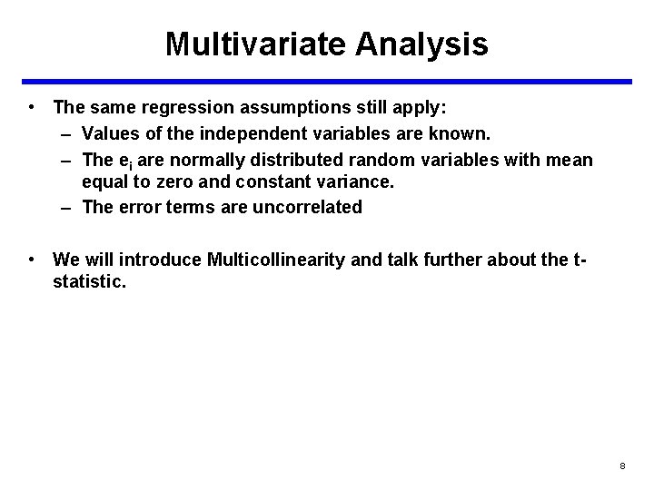
Multivariate Analysis • The same regression assumptions still apply: – Values of the independent variables are known. – The ei are normally distributed random variables with mean equal to zero and constant variance. – The error terms are uncorrelated • We will introduce Multicollinearity and talk further about the tstatistic. 8

Multivariate Analysis • What do the coefficients, (b 1, b 2, …, bk) represent? • In a simple linear model with one X, we would say b 1 represents the change in Y given a one unit change in X. • In the multivariate model, there is more of a conditional relationship. – Y is determined by the combined effects of all the X’s. • In the multivariate model, we say that b 1 represents the marginal change in Y given a one unit change in X 1, while holding all the other Xi constant. • In other words, the value of b 1 is conditional on the presence of the other independent variables in the equation. 9

Multicollinearity • One factor in the ability of the regression coefficient to accurately reflect the marginal contribution of an independent variable is the amount of independence between the independent variables. • If Xi and Xj are statistically independent, then a change in Xi has no correlation to a change in Xj. • Usually, however, there is some amount of correlation between variables. • Multicollinearity occurs when Xi and Xj are related to each other. • When this happens, there is an “overlap” between what Xi explains about Y and what Xj explains about Y. This makes it difficult to determine the true relationship between Xi and Y, and Xj and Y. 10

Multicollinearity • One of the ways we can detect multicollinearity is by observing the regression coefficients. • If the value of b 1 changes significantly from an equation with X 1 only to an equation with X 1 and X 2, then there is a significant amount of correlation between X 1 and X 2. • A better way of detecting this is by looking at a pairwise correlation matrix. • The values in the pairwise correlation matrix represent the “r” values between the variables. • We will define variables as “multicollinear, ” or highly correlated, when r 0. 7 11

Multicollinearity • In general, multicollinearity does not necessarily affect our ability to get a good fit, nor does it affect our ability to obtain a good prediction, provided that we maintain the multicollinear relationship between variables. • How do we determine that relationship? • Run simple linear regression between the two correlated variables. • For example, if Cost = 23 + 3. 5*Weight + 17*Speed and we find that weight and speed are highly correlated, then we run a regression between the variables Weight and Speed to determine their relationship. – Say, Weight = 8. 3+1. 2*Speed • We can still use our previous CER as long as our inputs for Weight and Speed follow this relationship (approximately). • If the relationship is not maintained, then we are probably estimating something different from what’s in our data set. 12

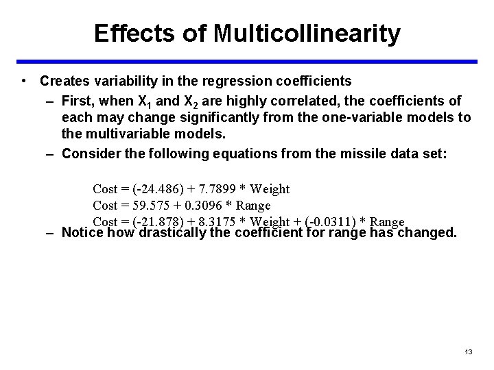
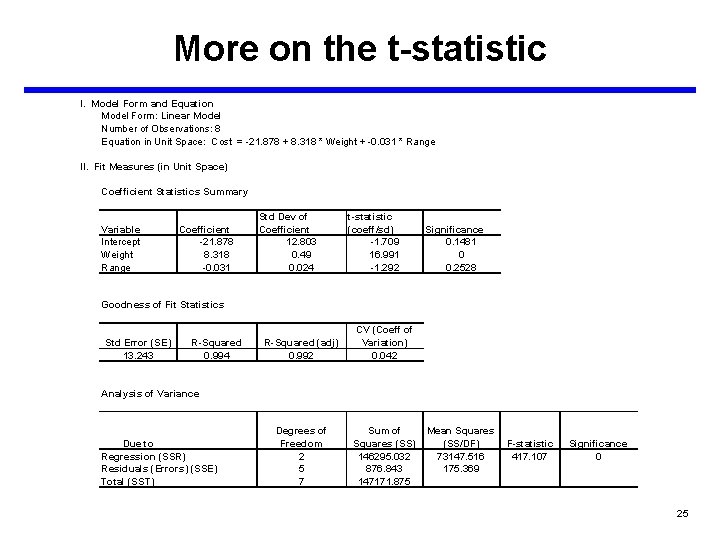
Effects of Multicollinearity • Creates variability in the regression coefficients – First, when X 1 and X 2 are highly correlated, the coefficients of each may change significantly from the one-variable models to the multivariable models. – Consider the following equations from the missile data set: Cost = (-24. 486) + 7. 7899 * Weight Cost = 59. 575 + 0. 3096 * Range Cost = (-21. 878) + 8. 3175 * Weight + (-0. 0311) * Range – Notice how drastically the coefficient for range has changed. 13

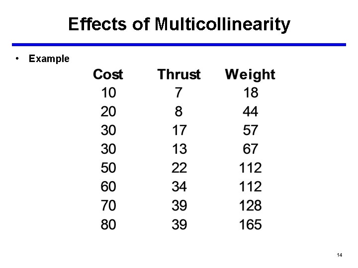
Effects of Multicollinearity • Example 14

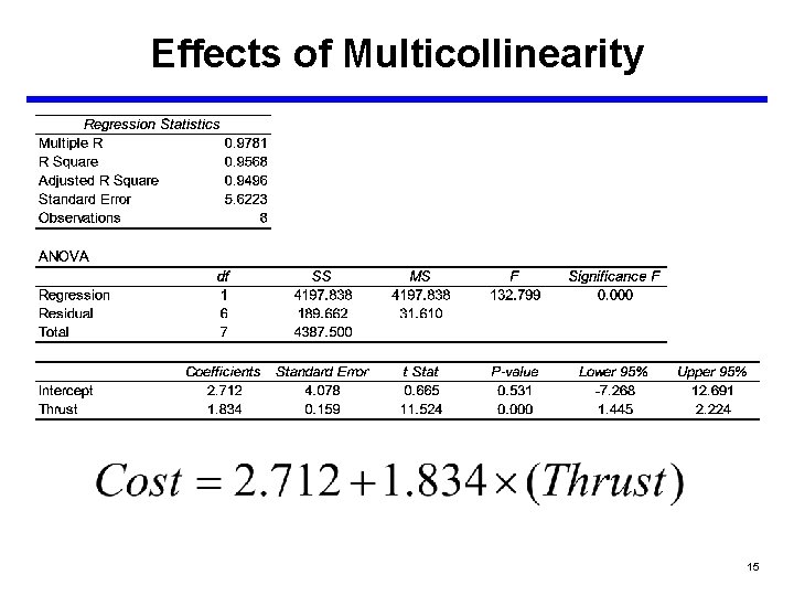
Effects of Multicollinearity 15

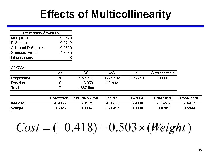
Effects of Multicollinearity 16

Effects of Multicollinearity 17

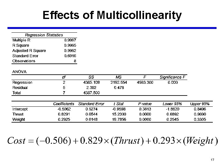
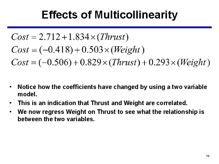
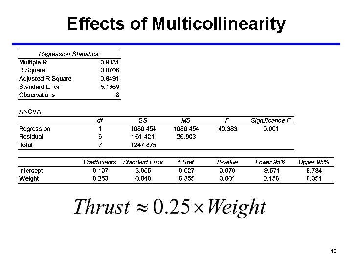
Effects of Multicollinearity • Notice how the coefficients have changed by using a two variable model. • This is an indication that Thrust and Weight are correlated. • We now regress Weight on Thrust to see what the relationship is between the two variables. 18

Effects of Multicollinearity 19

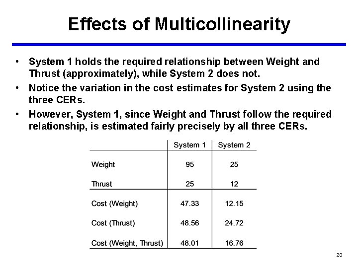
Effects of Multicollinearity • System 1 holds the required relationship between Weight and Thrust (approximately), while System 2 does not. • Notice the variation in the cost estimates for System 2 using the three CERs. • However, System 1, since Weight and Thrust follow the required relationship, is estimated fairly precisely by all three CERs. 20

Effects of Multicollinearity • When multicollinearity is present we can no longer make the statement that b 1 is the change in Y for a unit change in X 1 while holding X 2 constant. – The two variables may be related in such a way that precludes varying one while the other is held constant. – For example, perhaps the only way to increase the range of a missile is to increase the amount of the propellant, thus increasing the missile weight. • One other effect is that multicollinearity might prevent a significant cost driver from entering the model during model selection. 21

Remedies for Multicollinearity? • Drop a variable and ignore an otherwise good cost driver? – Not if we don’t have to. • Involve technical experts. – Determine if the model is correctly specified. • Combine the variables by multiplying or dividing them. • Rule of Thumb for determining if you have multicollinearity: – Widely varying coefficients – Correlation Matrix: » r 0. 3 No Problem » 0. 3 r 0. 7 Gray Area » r 0. 7 Problems Exist 22

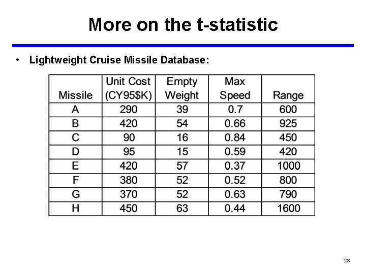
More on the t-statistic • Lightweight Cruise Missile Database: 23

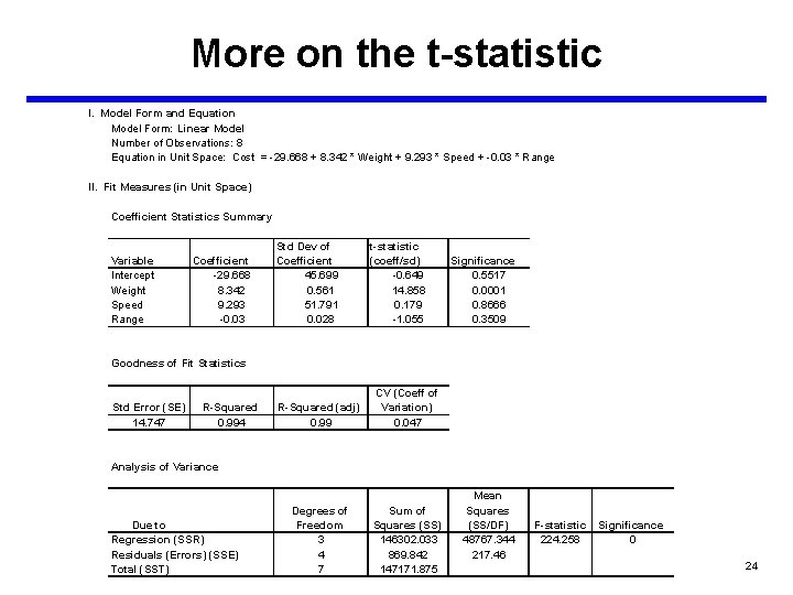
More on the t-statistic I. Model Form and Equation Model Form: Linear Model Number of Observations: 8 Equation in Unit Space: Cost = -29. 668 + 8. 342 * Weight + 9. 293 * Speed + -0. 03 * Range II. Fit Measures (in Unit Space) Coefficient Statistics Summary Variable Intercept Weight Speed Range Coefficient -29. 668 8. 342 9. 293 -0. 03 Std Dev of Coefficient 45. 699 0. 561 51. 791 0. 028 t-statistic (coeff/sd) -0. 649 14. 858 0. 179 -1. 055 Significance 0. 5517 0. 0001 0. 8666 0. 3509 Goodness of Fit Statistics Std Error (SE) 14. 747 R-Squared 0. 994 R-Squared (adj) 0. 99 CV (Coeff of Variation) 0. 047 Degrees of Freedom 3 4 7 Sum of Squares (SS) 146302. 033 869. 842 147171. 875 Analysis of Variance Due to Regression (SSR) Residuals (Errors) (SSE) Total (SST) Mean Squares (SS/DF) 48767. 344 217. 46 F-statistic 224. 258 Significance 0 24

More on the t-statistic I. Model Form and Equation Model Form: Linear Model Number of Observations: 8 Equation in Unit Space: Cost = -21. 878 + 8. 318 * Weight + -0. 031 * Range II. Fit Measures (in Unit Space) Coefficient Statistics Summary Variable Intercept Weight Range Coefficient -21. 878 8. 318 -0. 031 Std Dev of Coefficient 12. 803 0. 49 0. 024 t-statistic (coeff/sd) -1. 709 16. 991 -1. 292 Significance 0. 1481 0 0. 2528 Goodness of Fit Statistics Std Error (SE) 13. 243 R-Squared 0. 994 R-Squared (adj) 0. 992 CV (Coeff of Variation) 0. 042 Degrees of Freedom 2 5 7 Sum of Squares (SS) 146295. 032 876. 843 147171. 875 Analysis of Variance Due to Regression (SSR) Residuals (Errors) (SSE) Total (SST) Mean Squares (SS/DF) 73147. 516 175. 369 F-statistic 417. 107 Significance 0 25

Selecting the Best Model 26

Choosing a Model • • We have seen what the linear model is, and explored it in depth We have looked briefly at how to generalize the approach to non-linear models You may, at this point, have several significant models from regressions – One or more linear models, with one or more significant variables – One or more non-linear models Now we will learn how to choose the “best model” 27

Steps for Selecting the “Best Model” • You should already have rejected all non-significant models first – If the F statistic is not significant • You should already have stripped out all non-significant variables and made the model “minimal” – Variables with non-significant t statistics were already removed • Select “within type” based on R 2 • Select “across type” based on SSE We will examine each in more detail… 28

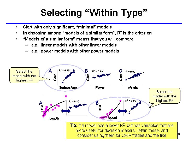
Selecting “Within Type” Start with only significant, “minimal” models In choosing among “models of a similar form”, R 2 is the criterion “Models of a similar form” means that you will compare – e. g. , linear models with other linear models – e. g. , power models with other power models Cost B Surface Area Power Weight Select the model with the highest R 2 B Cost A C Cost A Select the model with the highest R 2 Cost • • • Length Speed Tip: If a model has a lower R 2, but has variables that are more useful for decision makers, retain these, and consider using them for CAIV trades and the like 29

Selecting “Across Type” • • • Start with only significant, “minimal” models In choosing among “models of a different form”, the SSE in unit space is the criterion “Models of a different form” means that you will compare: – e. g. , linear models with non-linear models – e. g. , power models with logarithmic models We must compute the SSE by: – Computing Ŷ in unit space for each data point – Subtracting each Ŷ from its corresponding actual Y value – Sum the squared values, this is the SSE An example follows… Warning: We cannot use R 2 to compare models of different forms because the R 2 from the regression is computed on the transformed data, and thus is distorted by the transformation 30