5 Regression Analysis Linear Regression Model simple regression

第 5回　回帰モデル Regression Analysis • 回帰モデル Linear Regression Model –単回帰モデル、重回帰モデル –simple regression, multivariate regression –非線形式の回帰分析 nonlinear regression • 最小二乗法（記述統計） Least square method –回帰式の適合度のチェック（分散分析）ANOVA: analysis of variance to check fitness • 最小二乗推定量の性質（推測統計） –パラメータ推定量の不偏性 Unbiased estimator –パラメータ推定量の確率分布とｔ検定 Distribution of the estimator and Student’s t test 1

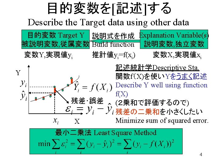
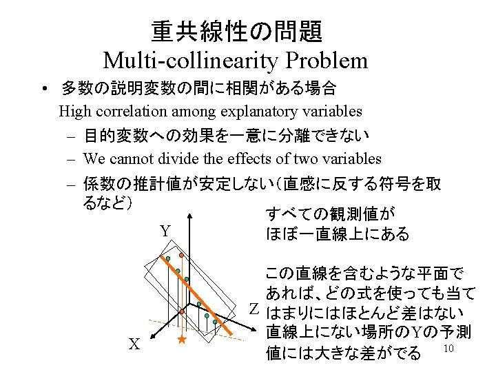
回帰モデル Regression Model • ある変数の値を、別の変数を用いて説明 • Explain target variable by other variable(s) based on correlation among them. 目的変数 Target Y 説明式を作成 Explanation Variable(s) 被説明変数, 従属変数 Build function 説明変数, 独立変数 変数Y, 実現値yi 推計値yi=f(xi) 変数X, 実現値xi Y Y Z X X 2

記述統計学と推測統計学 Descriptive Statistics, Inference Statistics Descriptive Statistics 母集団の データ Data in Population 多数データの 数学的要約･記述 Summary of many numbers Inference Statistics 無作為抽出 Random sampling 標本集団 (仮想的) のデータ 母集団 samples population 母数(parameter) 確率的推測･記述 inference 少数データの 数学的要約･記述 Summary of smaller numbers 3

行列を用いた重回帰式の計算例 lm(formula = strong ~ chem. A + chem. B) Coefficients: (Intercept) chem. A chem. B 39. 728 6. 433 1. 750 8

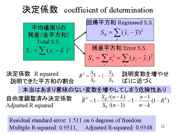
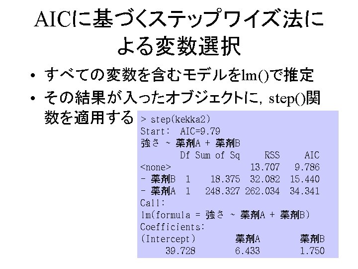
Call: lm(formula = 強さ ~ 薬剤A) Rによる計算例 Residuals: #データフレームを作成する Min 1 Q Median 3 Q Max concrete <- data. frame(-2. 1111 -1. 3444 -0. 8111 0. 8222 3. 6556 Call: + strg=c(40. 0, 45. 8, 53. 0, 42. 3, 46. 7, 54. 1, 44. 2, 47. 1, 58. 0), lm(formula = 強さ ~ 薬剤A + 薬剤B) Coefficients: + chem. A =c(0, 1, 2, 0, 1, 2), Estimate Std. Error t value Pr(>|t|) + chem. B =c(0, 0, 0, 1, 1, 1, 2, 2, 2) Residuals: (Intercept) 41. 478 1. 128 36. 761 2. 86 e-09 *** ) Min 1 Q Median 3 Q Max 0. 000154 *** 薬剤A 6. 433 0. 874 7. 361 -2. 5611 -0. 3611 0. 2722 0. 8222 1. 9056 #データフレームから変数に代入(付置)する --streng <-concrete$strg Signif. codes: 0 ‘***’ 0. 001 ‘**’ 0. 01 ‘*’ 0. 05 ‘. ’ 0. 1 ‘ ’ Coefficients: 1 chemical. A <- concrete$chem. A Estimate Std. Error t value Pr(>|t|) chemical. B <- concrete$chem. B (Intercept) 39. 7278 1. 78 e-08 *** Residual standard error: 1. 0076 2. 141 on 39. 426 7 degrees of freedom #単回帰分析の結果をkekka 1に入れ，その概要を出力 薬剤A 6. 4333 0. 8856, 0. 6171 Adjusted 10. 426 4. 56 e-05 *** 0. 8692 Multiple R-squared: 薬剤B 1. 7500 on 1 and 0. 6171 0. 0297 * kekka 1 <- lm(streng~chemical. A) F-statistic: 54. 18 7 DF, 2. 836 p-value: 0. 0001545 --summary(kekka 1) Signif. codes: 0 ‘***’ 0. 001 ‘**’ 0. 01 ‘*’ 0. 05 ‘. ’ 0. 1 ‘ ’ #重回帰分析の結果をkekka 2に入れ，その概要を出力 1 kekka 2 <- lm(streng~chemical. A+chemical. B) summary(kekka 2) Residual standard error: 1. 511 on 6 degrees of freedom Multiple R-squared: 0. 9511, Adjusted R-squared: 90. 9348 F-statistic: 58. 37 on 2 and 6 DF, p-value: 0. 0001168

同じ正規母集団からの 2つの分散とその比 Variances of two sample sets from one population 正規分布母集団 Normal Distributed Population Sample set B Sample set A 不偏分散推定量 Unbiased Variance 分散の比 Ratio of Variances 分散の比は、F分布に従う。 Ratio of the two variances obeys F distribution. 13

同じ母集団からの 2つの分散とその比 Variances of two sample sets from one population #母集団分布を仮定する（正規分布）　4. 4. 5 var. A<-numeric(length=10000); var. B<-numeric(length=10000) var. AB <-numeric(length=10000); na<-20; nb<-10 for(i in 1: 10000){ sampleset. A　<-　rnorm(n=na+1, mean=0, sd=1) #generate sampleset. B　<-　rnorm(n=nb+1, mean=0, sd=1) #generate sampleset var. A [i] <- var(sampleset. A) # store Variance A var. B [i] <-var(sampleset. B) # store Variance B var. AB[i] <- var(sampleset. A) / var(sampleset. B) } hist(var. A, freq=FALSE, border="blue") curve(dchisq(x*na, na)*na, add=TRUE) hist(var. B, freq=FALSE, border="red", add=TRUE) curve(dchisq(x*nb, nb)*nb, add=TRUE) mean(var. A); var(var. A) # Variance A mean(var. B); var(var. B) # Variance B 14

同じ母集団からの 2つの分散とその比 Variances of two sample sets from one population #Distribution of the ratio of the two variances calculated from samples mean(var. AB); var(var. AB) # Ratio of two Variances hist(var. AB, freq=FALSE, border="green") #histogram of the ratio of two variances curve(df(x, na, nb), add=TRUE) # theoretical distribution (F with na and nb DF) 同じ母集団からの 2つの標 本から分散を計算し、その 比をとったものは、F分布に 従う。 Ratio of the two variances of two sample sets from one population obeys F distribution. 15

回帰による記述（説明）力の検定 ANOVA Test of overall fitness 回帰平方和が誤差平方和に比べ、大きな意味を持っているか？ Does RSS have remarkable meaning comparing to ESS? 帰無仮説：回帰平方和は誤差平方和と同程度の大きさ （回帰式は、誤差に比べて大きな説明力はない） Null Hypothesis: RSS have similar meaning with ESS. (Ratio of Two Variances originated from same population obeys to F-distribution) 対立仮説：回帰平方和は誤差平方和より大きい 　（回帰式によって誤差よりもかなり大きい部分が説明できた） Alternative Hypothesis. : RSS have larger meaning than ESS. 16

回帰による記述（説明）力の検定例 帰無仮説：回帰平方和は誤差平方和と同程度の大きさ （回帰式は、誤差に比べて大きな説明力はない） Rejected (棄却） Null Hypothesis: RSS have similar meaning with ESS. (Ratio of Two Variances originated from same population obeys to F-distribution) 対立仮説：回帰平方和は誤差平方和より大きい採択Approved 　（回帰式によって誤差よりもかなり大きい部分が説明できた） Alternative Hypothesis. : RSS have larger meaning than ESS. Multiple R-squared: 0. 9511, Adjusted R-squared: 0. 9348 17 F-statistic: 58. 37 on 2 and 6 DF, p-value: 0. 0001168

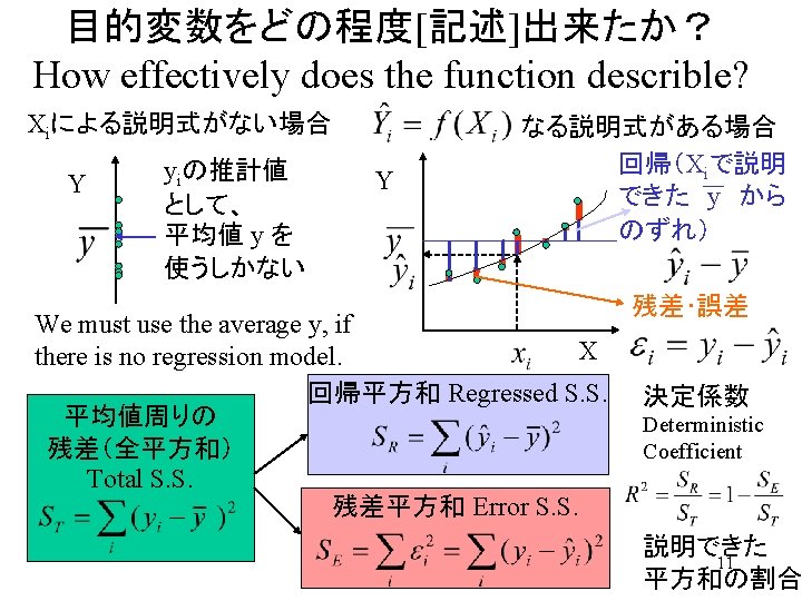
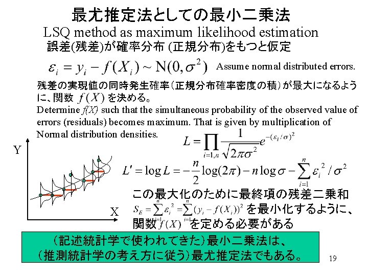
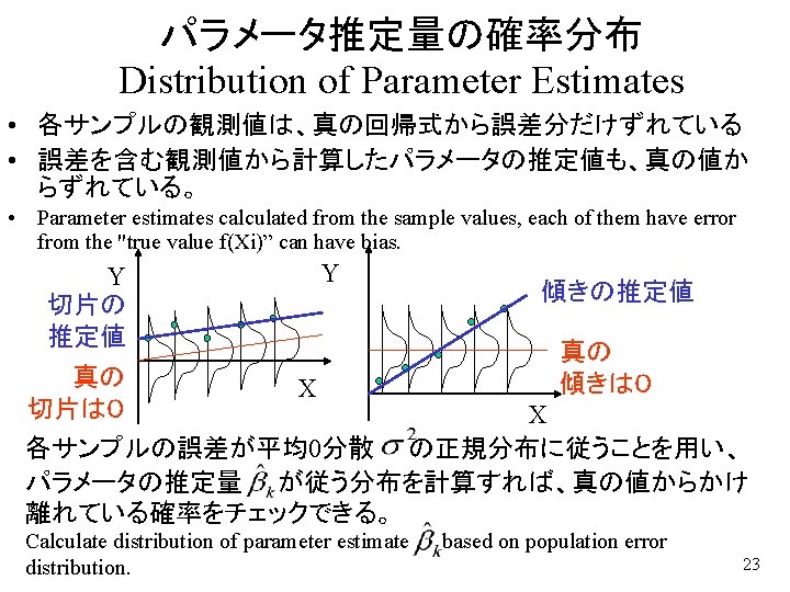
推測統計学の導入（母集団の性質の推測） Inference Statistics in Regression Analysis 各観測値は、真の値を中心にばらついていた Each observed yi distributes around yi=f(Xi). 誤差が正規分布に従うと仮定 Assume Normal distribution for error (in Population) Y Y 残差･誤差 X X 関数形　　　　を決めると、誤差の実現値　　　　　　が決まる。 それらが正規分布のもとで発生する確率を計算できる。 Once you assume f(X), you obtain the realized value of errors 18 , then you can estimate the probability of occurrence of them.

Trial in R # data making for X x 1 <- rep(1, 100) x 2 <- rep(seq(0, 9), 10) x 3 <- numeric(100) for(i in 0: 9){ for(j in 1: 10){x 3[i*10+j] <- i} } # X <- cbind(x 1, x 2, x 3) Xt <- t(X) Xt. X <- Xt %*% X Xt. Xinv <- solve(Xt. X) beta <- c(10, 1, 1) # make one sample set Y Y <- X %*% beta + rnorm(100, 0, 1) # library(rgl) plot 3 d(x 2, x 3, Y) # regression rslt <- lm(Y ~ x 2 + x 3) summary(rslt) objects(rslt) rslt$coefficients rslt$residuals aicr <- AIC(rslt) devia <- aicr +rslt$rank resid <- Y - X %*% rslt$coefficients LL <- sum(log(dnorm(resid, 0, 1))) ess <- t(resid) %*% resid 20

Parameter Estimation ## estimation of beta 2 # produce other values for beta 2 and check residuals bet 2 <-numeric(200) essq <- numeric(200) LLik <- numeric(200); Llik <- rep(0, 200) for(i in 1: 200) { bet 2[i] <- i*0. 01 resid <- Y - X %*% c(10, bet 2[i], 1) essq[i] <- t(resid) %*% resid LLik[i] <- sum(log(dnorm(resid, 0, 1))) } plot(bet 2, essq) # Sum of Squared Errors plot(bet 2, LLik) # Log Likelihood 21

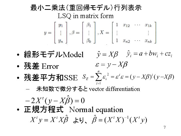
最小二乗推定量の確率分布 Distribution of Least-square Estimates • 最小二乗推定量の行列表示 • 観測値の誤差構造 – これらより、 – Where, 　　　　is not stochastic variables but fixed value. 不偏性 Unbiasedness – Ε takes both negative values and positive values with same probability. Average E[ε]=0 – Average of Estimates equal to true value. 24

最小二乗推定量の確率分布(2) Distribution of Least-square Estimates(2) • 最小二乗推定量の確率分布 • If 　 obeys to Normal distribution, the linear ε function of ε also obeys to a Normal Distribution. パラメータの分散共分散行列 Covariance Matrix of Parameter estimates j番目の対角要素 • j番目のパラメータの分散： • 誤差の母分散　　はわからないから、残差平方和からの分 散推定値で代用 25

最小二乗推定量の確率分布(2) Distribution of Least-square Estimates(2) • Probability of Normal distributing bias – Based on estimate value of variance, – instead of real variance→t distibution • ｔ statistics – t-distribution of d. f. of n-k – Under Null Hypothesis: 　(There is no effect of j-th variable) 　　　　　　　　obeys t-distribution of d. f. =n-k Coefficients: Estimate Std. Error t value Pr(>|t|) (Intercept) 39. 7278 1. 0076 39. 426 1. 78 e-08 *** 薬剤A 6. 4333 0. 6171 10. 426 4. 56 e-05 *** 薬剤B 1. 7500 0. 6171 2. 836 0. 0297 * 26

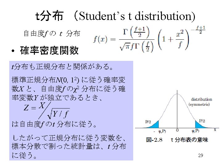
正規母集団からの標本値の確率分布 Mean and Variance of one sample set from one population 正規分布母集団 Normal Distributed Population Sample set 不偏分散推定量 Unbiased Variance 不偏標準偏差による標準化　 Standardized by Unbiased Estimator t分布に従う。 Standardized Y obeys Student’s t distribution. 27

不偏分散推定量で標準化したサンプル値の分布 Distribution of Value after standardization by unbiased SD estimator smp. X<-numeric(length=1000) sd. X<-numeric(length=1000) smp. Y<- numeric(length=1000) m 1<-0; sg 1<-sqrt(10) #Monte Carlo Simulation for(i in 1: 1000){ X <- rnorm(n=10, mean=m 1, sd=sg 1) smp. X[i] <- (X[1]-mean(X)) sd. X[i]<-sd(X) smp. Y[i]<- smp. X[i]/sd. X[i] } #Distribution of Y variable curve(dnorm(x, mean=0, sd=1), from=-3. 5, to=3. 5) hist(smp. Y, freq=FALSE, add=TRUE) curve(dt(x, 9), col = "violet", add = TRUE) 28

Produce one set of # data making for X x 1 <- rep(1, 100) x 2 <- rep(seq(0, 9), 10) x 3 <- numeric(100) for(i in 0: 9){ for(j in 1: 10){x 3[i*10+j] <- i} } X <- cbind(x 1, x 2, x 3) Xt <- t(X) Xt. X <- Xt %*% X Xt. Xinv <- solve(Xt. X) beta <- c(10, 1, 1) # make one sample set Y Y <- X %*% beta + rnorm(100, 0, 1) # regression once rslt <- lm(Y ~ x 2 + x 3) summary(rslt) objects(rslt) rslt$coefficients rslt$residuals aicr <- AIC(rslt) devia <- aicr +rslt$rank resid <- Y - X %*% rslt$coefficients LL <- sum(log(dnorm(resid, 0, 1))) ess <- t(resid) %*% resid 30

Monte Carlo Simulation # data making for X x 1 <- rep(1, 100) x 2 <- rep(seq(0, 9), 10) x 3 <- numeric(100) for(i in 0: 9){ for(j in 1: 10){x 3[i*10+j] <- i} } # X <- cbind(x 1, x 2, x 3) Xt <- t(X) Xt. X <- Xt %*% X Xt. Xinv <- solve(Xt. X) beta <- c(10, 1, 1) # prepare the storage for the estimated parameter(s) b 1 <- numeric(500) b 2 <- numeric(500) b 3 <- numeric(500) # Repeated Monte Carlo simulation for (i in 1: 500){ Y <- X %*% beta + rnorm(100, 0, 1) # regression rslt <- lm(Y ~ x 2 + x 3) brslt <- rslt$coefficients b 1[i] <- brslt[1] b 2[i] <- brslt[2] b 3[i] <- brslt[3] } # hist(b 1, freq=FALSE) resid <- Y - X %*% rslt$coefficients sigma. E<- sd(resid); V 1<- sigma. E*sqrt(Xt. Xinv[1, 1]) curve(dt((x-10)/V 1, 97)/V 1, add=TRUE) 31