Regression analysis Linear regression Logistic regression Relationship and

Regression analysis Linear regression Logistic regression

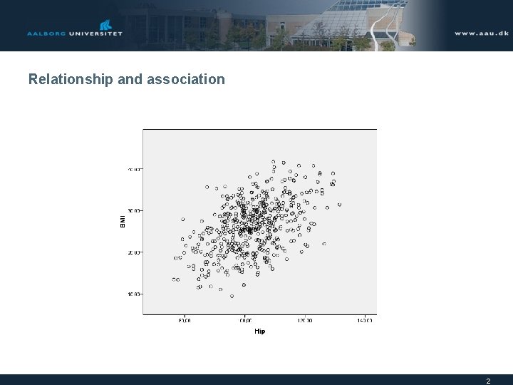
Relationship and association 2

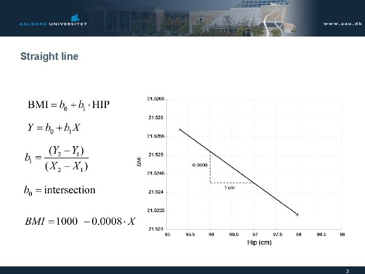
Straight line 3

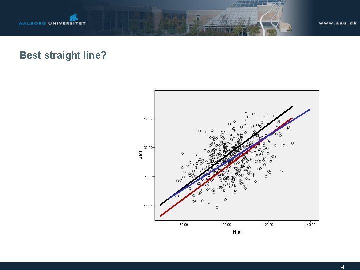
Best straight line? 4

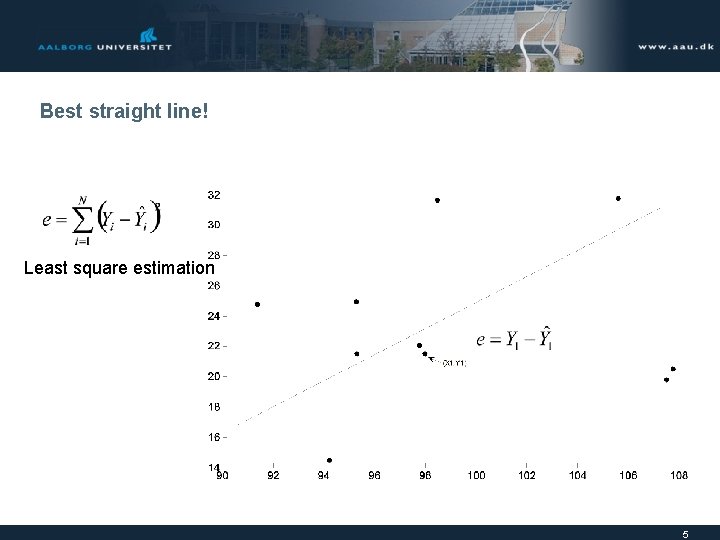
Best straight line! Least square estimation 5

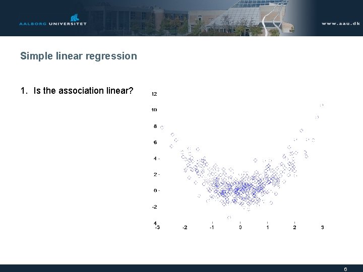
Simple linear regression 1. Is the association linear? 6

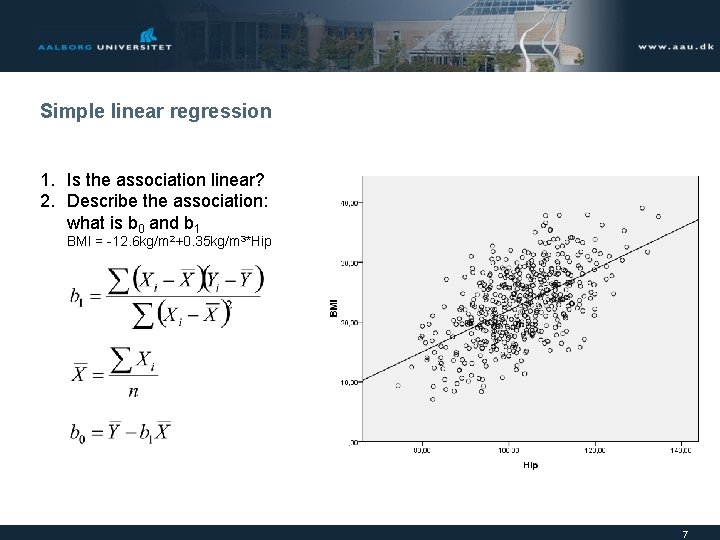
Simple linear regression 1. Is the association linear? 2. Describe the association: what is b 0 and b 1 BMI = -12. 6 kg/m 2+0. 35 kg/m 3*Hip 7

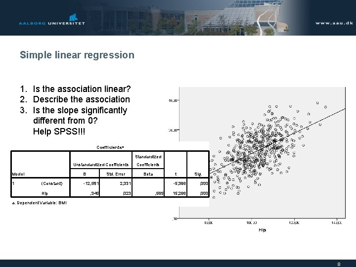
Simple linear regression 1. Is the association linear? 2. Describe the association 3. Is the slope significantly different from 0? Help SPSS!!! Coefficientsa Standardized Unstandardized Coefficients Model 1 B (Constant) Hip Std. Error -12, 581 2, 331 , 345 , 023 Coefficients t Beta , 565 Sig. -5, 396 , 000 15, 266 , 000 a. Dependent Variable: BMI 8

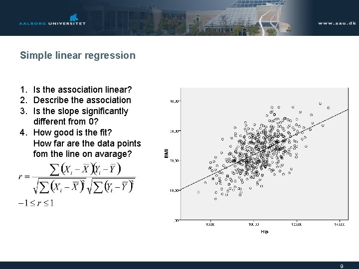
Simple linear regression 1. Is the association linear? 2. Describe the association 3. Is the slope significantly different from 0? 4. How good is the fit? How far are the data points fom the line on avarage? 9

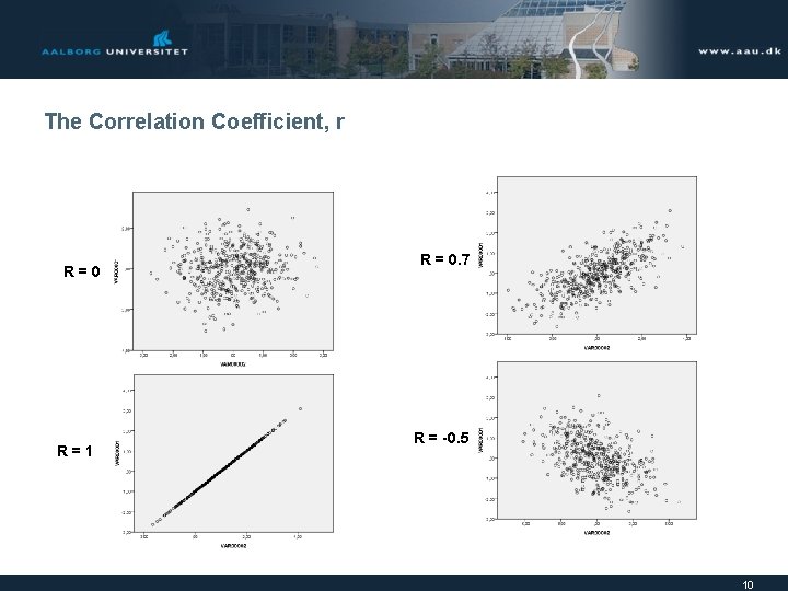
The Correlation Coefficient, r R=0 R=1 R = 0. 7 R = -0. 5 10

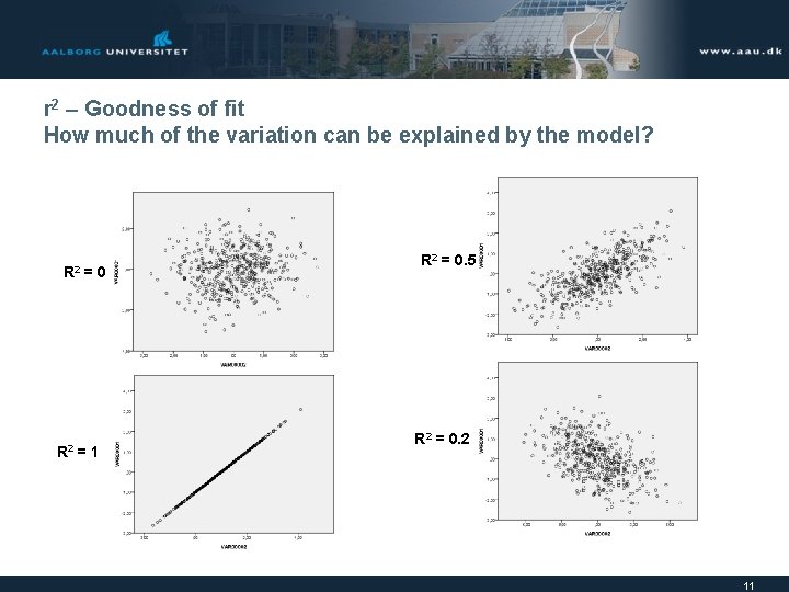
r 2 – Goodness of fit How much of the variation can be explained by the model? R 2 =0 =1 R 2 = 0. 5 R 2 = 0. 2 11

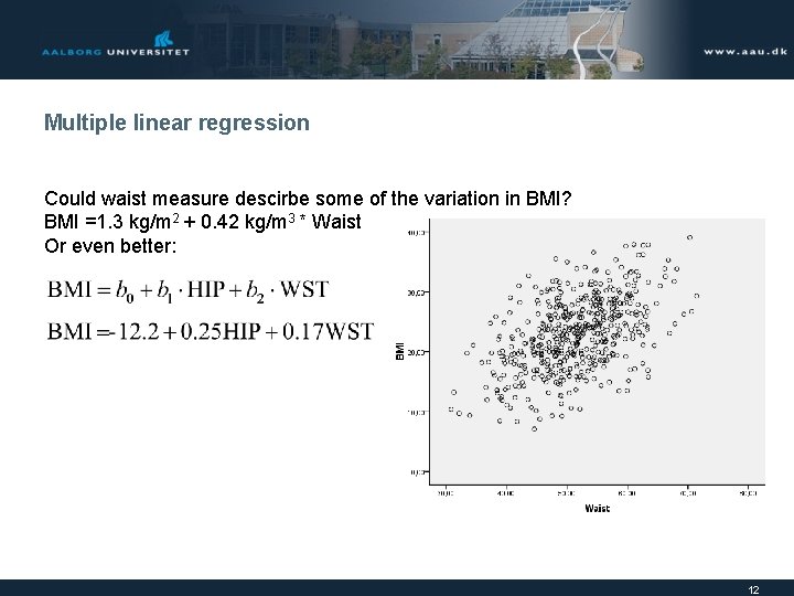
Multiple linear regression Could waist measure descirbe some of the variation in BMI? BMI =1. 3 kg/m 2 + 0. 42 kg/m 3 * Waist Or even better: 12

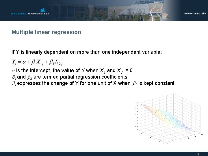
Multiple linear regression If Y is linearly dependent on more than one independent variable: is the intercept, the value of Y when X 1 and X 2 = 0 1 and 2 are termed partial regression coefficients 1 expresses the change of Y for one unit of X when 2 is kept constant 13

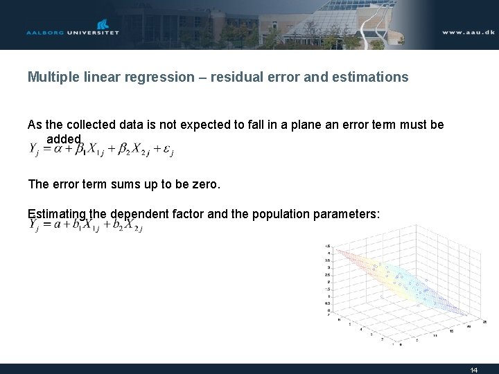
Multiple linear regression – residual error and estimations As the collected data is not expected to fall in a plane an error term must be added The error term sums up to be zero. Estimating the dependent factor and the population parameters: 14

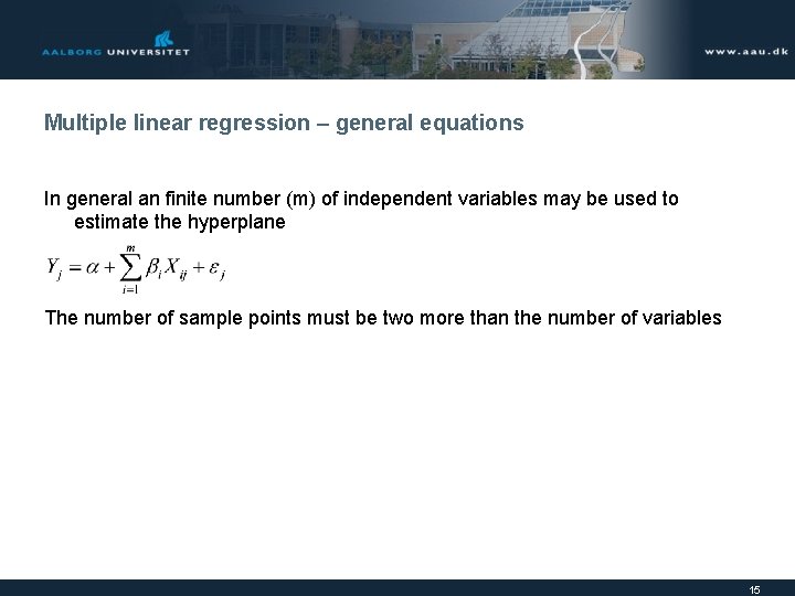
Multiple linear regression – general equations In general an finite number (m) of independent variables may be used to estimate the hyperplane The number of sample points must be two more than the number of variables 15

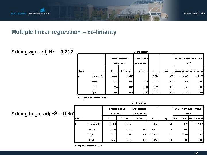
Multiple linear regression – co-liniarity Adding age: adj R 2 = 0. 352 Coefficientsa Model 1 Unstandardized Standardized 95, 0% Confidence Interval Coefficients for B B (Constant) Std. Error t Beta -9, 001 2, 449 Waist , 168 , 043 Hip , 252 Age -, 064 Sig. Lower Bound Upper Bound -3, 676 , 000 -13, 813 -4, 190 , 201 3, 923 , 000 , 084 , 252 , 031 , 411 8, 012 , 000 , 190 , 313 , 018 -, 126 -3, 492 , 001 -, 101 -, 028 a. Dependent Variable: BMI Coefficientsa Unstandardized Standardized 95, 0% Confidence Interval Coefficients for B Adding thigh: adj R 2 = 0. 352? Model 1 B (Constant) Waist Age Thigh Std. Error 3, 581 1, 784 , 168 , 043 -, 064 , 252 t Beta Sig. Lower Bound Upper Bound 2, 007 , 045 , 075 7, 086 , 201 3, 923 , 000 , 084 , 252 , 018 -, 126 -3, 492 , 001 -, 101 -, 028 , 031 , 411 8, 012 , 000 , 190 , 313 a. Dependent Variable: BMI 16

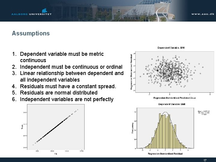
Assumptions 1. Dependent variable must be metric continuous 2. Independent must be continuous or ordinal 3. Linear relationship between dependent and all independent variables 4. Residuals must have a constant spread. 5. Residuals are normal distributed 6. Independent variables are not perfectly correlated with each other 17

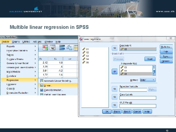
Multible linear regression in SPSS 18

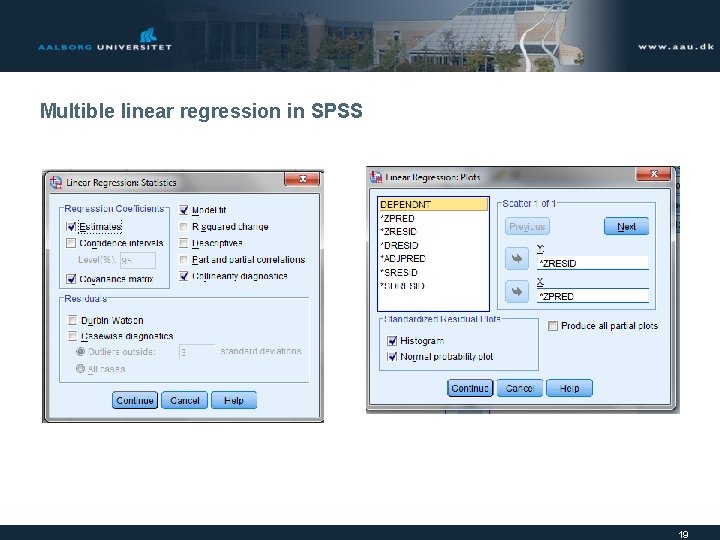
Multible linear regression in SPSS 19

Non-parametric correlation 20

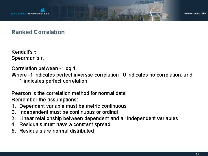
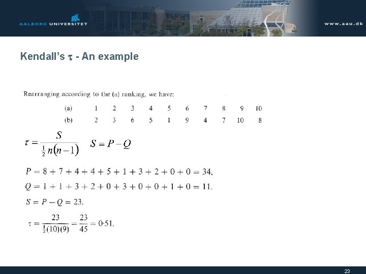
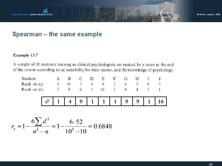
Ranked Correlation Kendall’s Spearman’s rs Correlation between -1 og 1. Where -1 indicates perfect inversse correlation , 0 indicates no correlation, and 1 indicates perfect correlation Pearson is the correlation method for normal data Remember the assumptions: 1. Dependent variable must be metric continuous 2. Independent must be continuous or ordinal 3. Linear relationship between dependent and all independent variables 4. Residuals must have a constant spread. 5. Residuals are normal distributed 21

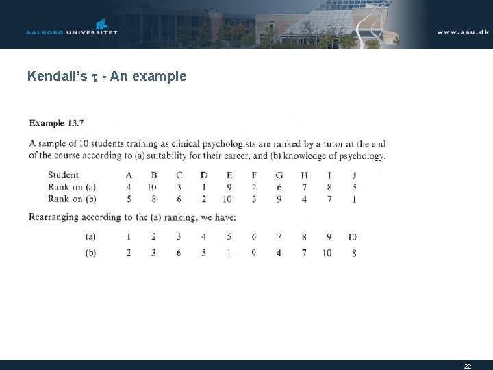
Kendall’s - An example 22

Kendall’s - An example 23

Spearman – the same example d 2 1 4 9 1 1 1 9 9 1 16 24

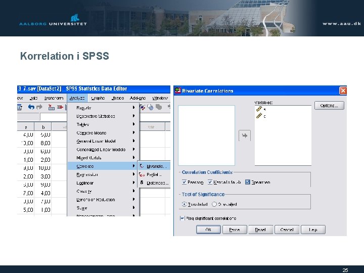
Korrelation i SPSS 25

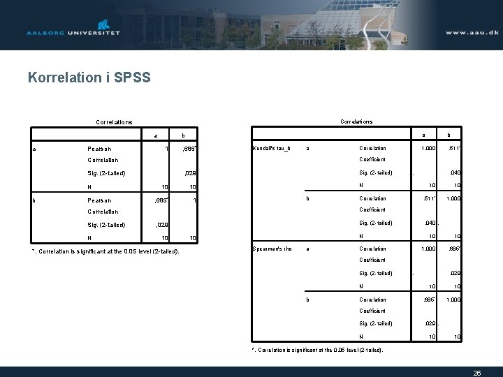
Korrelation i SPSS Correlations a a Pearson b 1 , 685* Kendall's tau_b a Sig. (2 -tailed) b Pearson Sig. (2 -tailed) , 029 10 10 N 1, 000 , 511* , 685* 1 . N b Correlation , 040 10 10 , 511* 1, 000 Coefficient Correlation Sig. (2 -tailed) b Coefficient Correlation N Correlation a Sig. (2 -tailed) , 029 10 *. Correlation is significant at the 0. 05 level (2 -tailed). , 040. N 10 Spearman's rho a Correlation 10 10 1, 000 , 685* Coefficient Sig. (2 -tailed) N b Correlation . , 029 10 10 , 685* 1, 000 Coefficient Sig. (2 -tailed) N , 029. 10 10 *. Correlation is significant at the 0. 05 level (2 -tailed). 26

Logistic regression 27

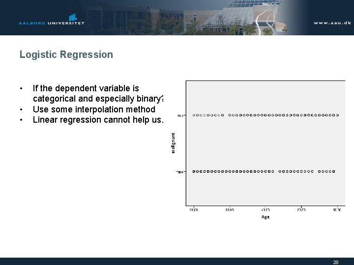
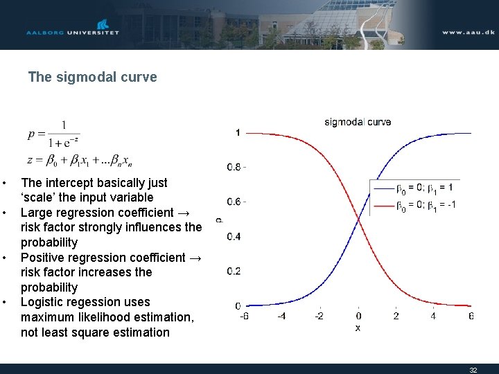
Logistic Regression • • • If the dependent variable is categorical and especially binary? Use some interpolation method Linear regression cannot help us. 28

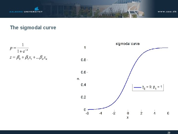
The sigmodal curve 29

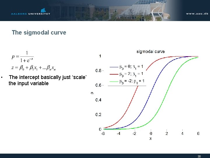
The sigmodal curve • The intercept basically just ‘scale’ the input variable 30

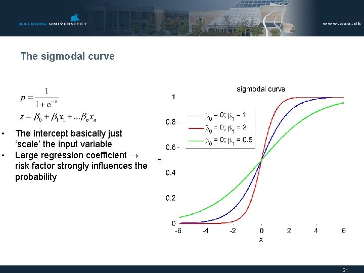
The sigmodal curve • • The intercept basically just ‘scale’ the input variable Large regression coefficient → risk factor strongly influences the probability 31

The sigmodal curve • • The intercept basically just ‘scale’ the input variable Large regression coefficient → risk factor strongly influences the probability Positive regression coefficient → risk factor increases the probability Logistic regession uses maximum likelihood estimation, not least square estimation 32

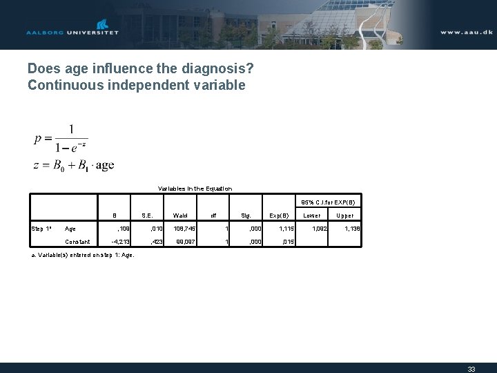
Does age influence the diagnosis? Continuous independent variable Variables in the Equation 95% C. I. for EXP(B) B Step 1 a Age Constant S. E. Wald df Sig. Exp(B) , 109 , 010 108, 745 1 , 000 1, 115 -4, 213 , 423 99, 097 1 , 000 , 015 Lower 1, 092 Upper 1, 138 a. Variable(s) entered on step 1: Age. 33

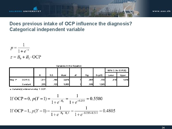
Does previous intake of OCP influence the diagnosis? Categorical independent variable Variables in the Equation 95% C. I. for EXP(B) B Step 1 a OCP(1) Constant S. E. Wald df Sig. Exp(B) -, 311 , 180 2, 979 1 , 084 , 733 , 233 , 123 3, 583 1 , 058 1, 263 Lower , 515 Upper 1, 043 a. Variable(s) entered on step 1: OCP. 34

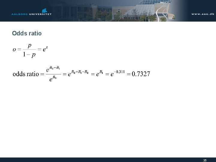
Odds ratio 35

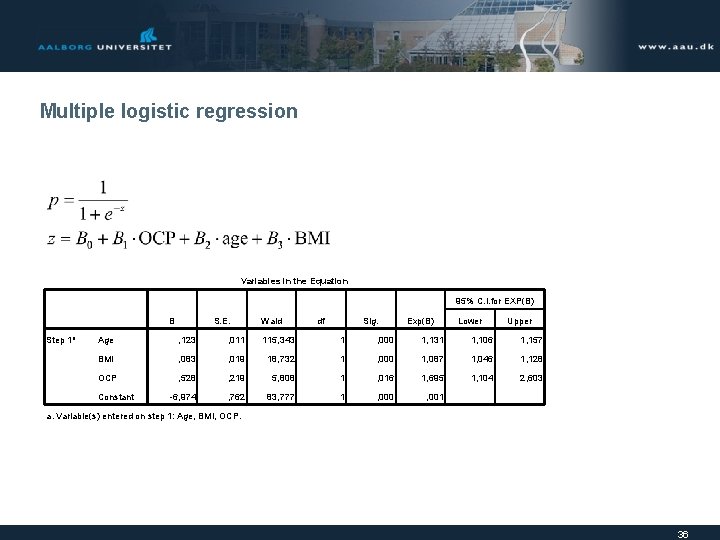
Multiple logistic regression Variables in the Equation 95% C. I. for EXP(B) B Step 1 a S. E. Wald df Sig. Exp(B) Lower Upper Age , 123 , 011 115, 343 1 , 000 1, 131 1, 106 1, 157 BMI , 083 , 019 18, 732 1 , 000 1, 087 1, 046 1, 128 OCP , 528 , 219 5, 808 1 , 016 1, 695 1, 104 2, 603 -6, 974 , 762 83, 777 1 , 000 , 001 Constant a. Variable(s) entered on step 1: Age, BMI, OCP. 36

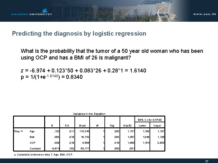
Predicting the diagnosis by logistic regression What is the probability that the tumor of a 50 year old woman who has been using OCP and has a BMI of 26 is malignant? z = -6. 974 + 0. 123*50 + 0. 083*26 + 0. 28*1 = 1. 6140 p = 1/(1+e-1. 6140) = 0. 8340 Variables in the Equation 95% C. I. for EXP(B) B Step 1 a S. E. Wald df Sig. Exp(B) Lower Upper Age , 123 , 011 115, 343 1 , 000 1, 131 1, 106 1, 157 BMI , 083 , 019 18, 732 1 , 000 1, 087 1, 046 1, 128 OCP , 528 , 219 5, 808 1 , 016 1, 695 1, 104 2, 603 -6, 974 , 762 83, 777 1 , 000 , 001 Constant a. Variable(s) entered on step 1: Age, BMI, OCP. 37

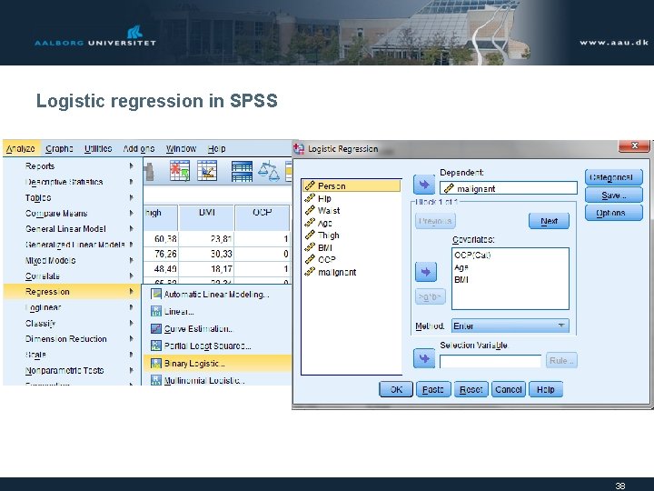
Logistic regression in SPSS 38

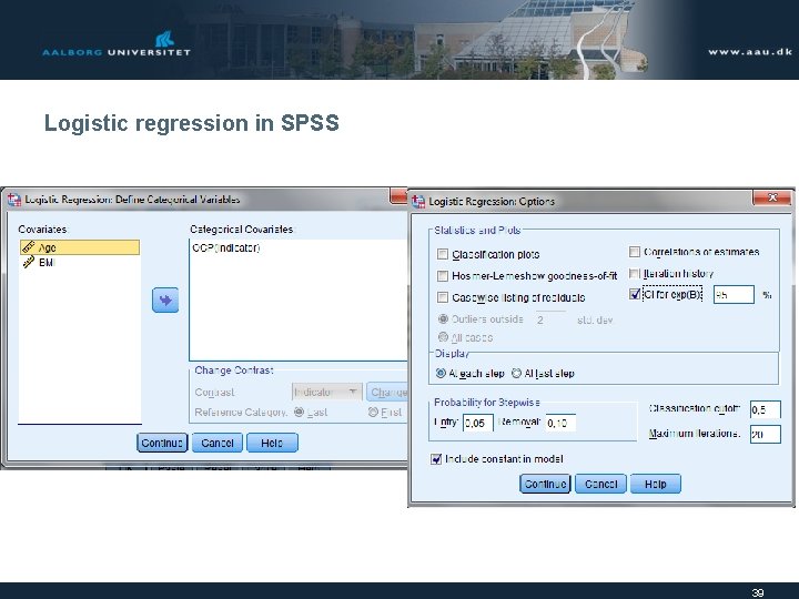
Logistic regression in SPSS 39