Multivariate Linear Regression Ph D Course Multivariate linear

Multivariate Linear Regression Ph. D Course

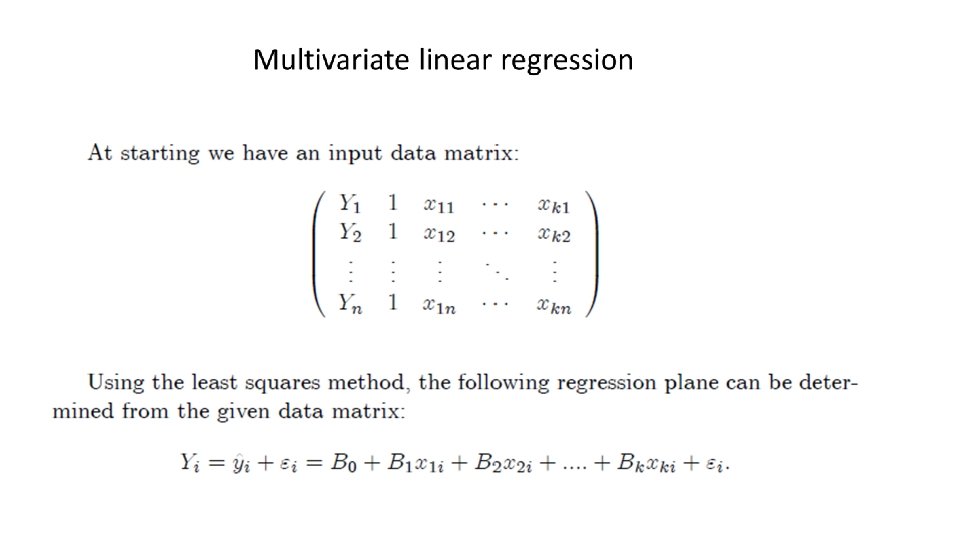
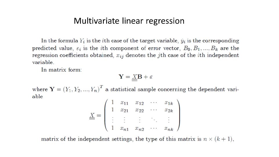
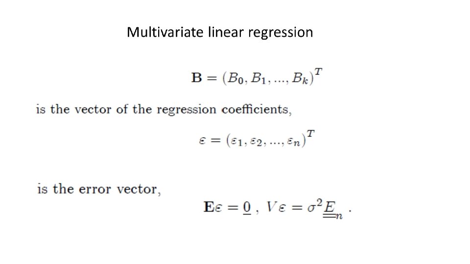
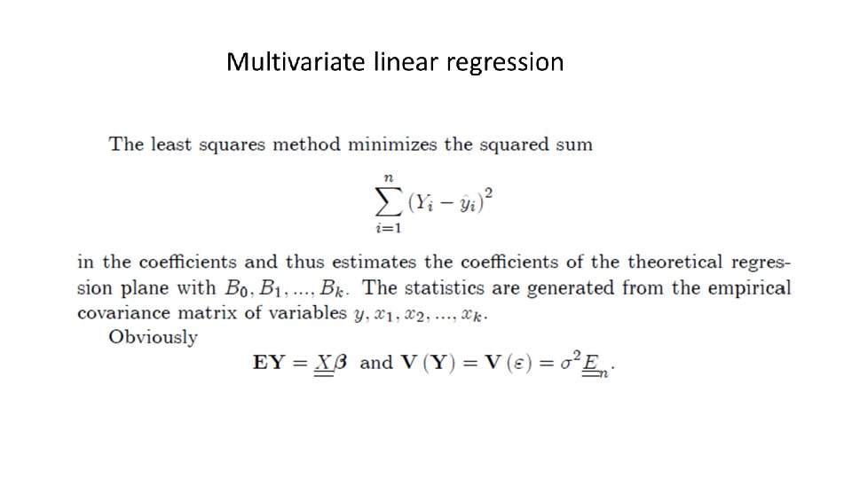
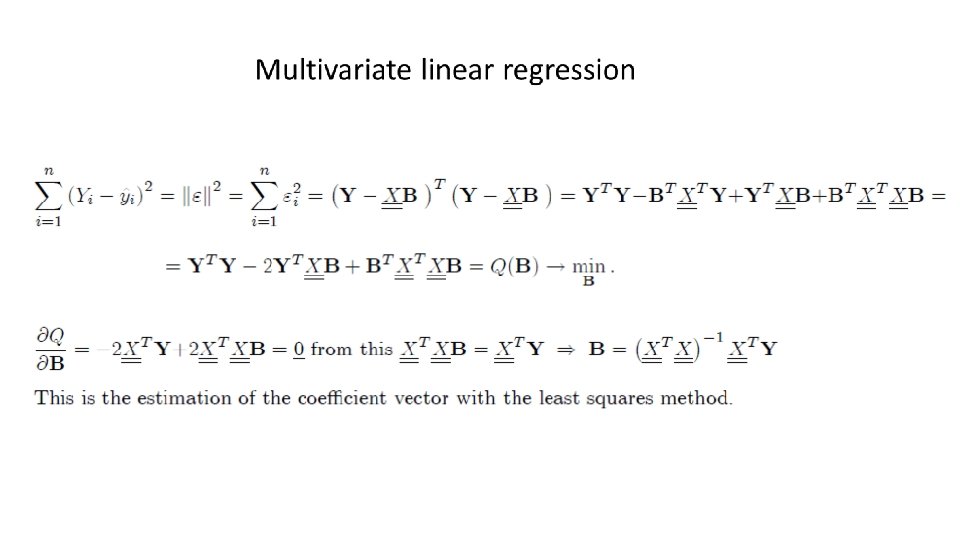
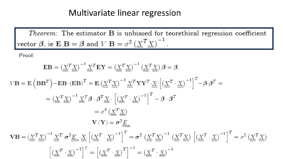
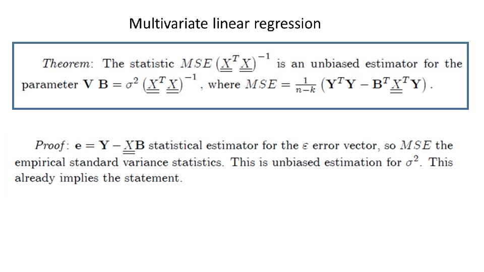
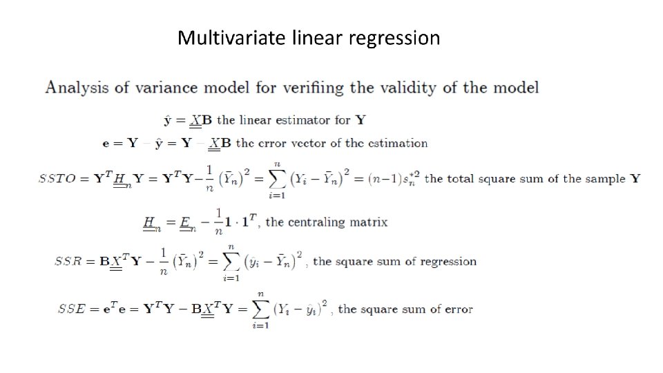
Multivariate linear regression

Geometrical interpretation of the partial correletion between x and y. The effect coused by z is eliminated at this correlation value between x and y.

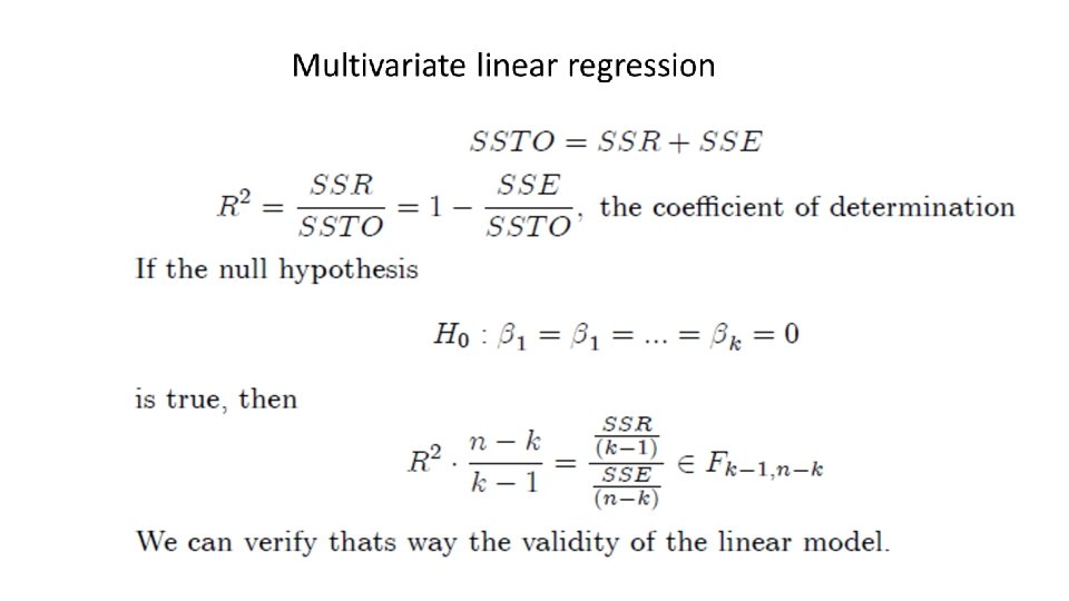
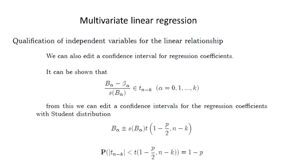
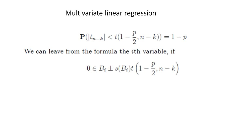
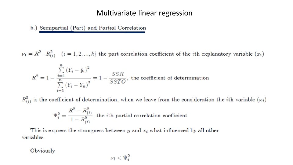
Partial F test

Partial F test

Partial F test

Partial F test

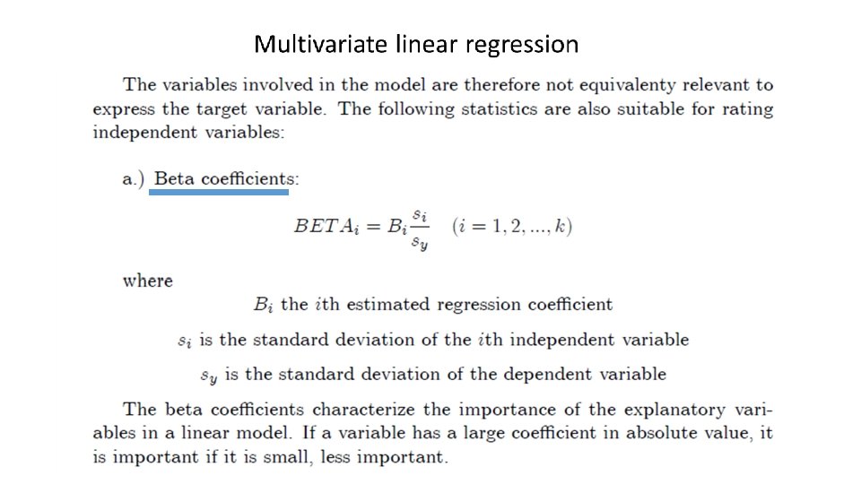
Automated modeling algorithms

Automated modeling algorithms

Automated modeling algorithms

Adjusted Coefficient of Determination You can use the adjusted coefficient of determination to determine how well a multiple regression equation fits the sample data. The adjusted coefficient of determination is closely related to the coefficient of determination (also known as R 2) that you use to test the results of a simple regression equation. p the number of the explanatory variables in the model

Adjusted Coefficient of Determination

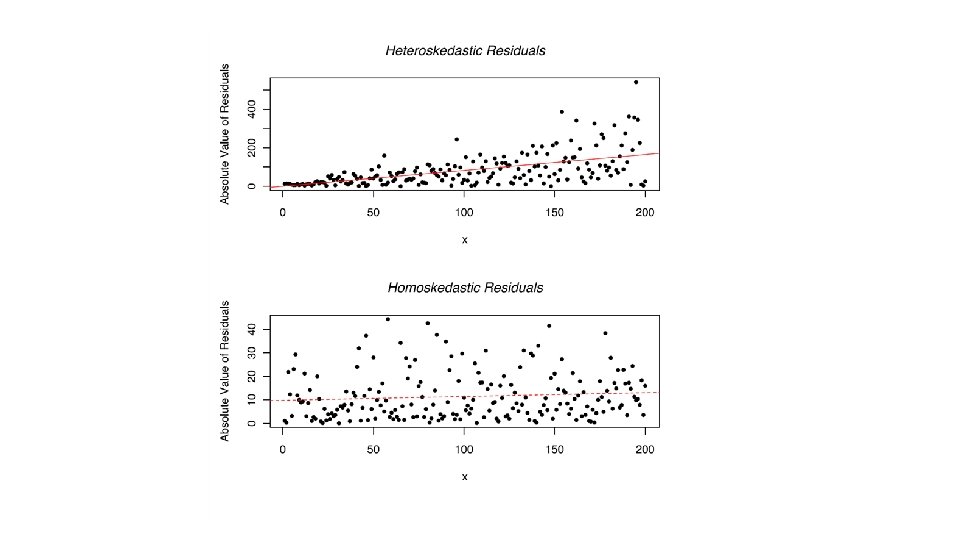
Heteroscedasticity in Regression Analysis You can see an example of this cone shaped pattern in the residuals by fitted value plot below. Note how the vertical range of the residuals increases as the fitted values increases.

Heteroscedasticity in Regression Analysis Possible types of scattering of residuals at zero level a. ) the scatter corresponds to the linear model, b. ) not the linear model belong to the residuals, c. ) the scatterings are not the same, d. ) the errors are not independent of each other.

Heteroscedasticity in Regression Analysis Heteroscedasticity means unequal scatter. In regression analysis, we talk about heteroscedasticity in the context of the residuals or error term. Specifically, heteroscedasticity is a systematic change in the spread of the residuals over the range of measured values. Heteroscedasticity is a problem because ordinary least squares (OLS) regression assumes that all residuals are drawn from a population that has a constant variance (homoscedasticity). To satisfy the regression assumptions and be able to trust the results, the residuals should have a constant variance.

Types of Residual Common Residual: Deleted Residual: Standardized Residual: Studendized Residual: When calculating the linear estimate, we do not calculate the "i" case, we "delete" it.

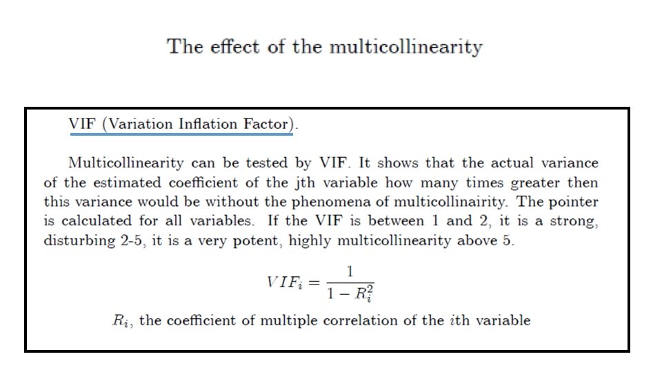
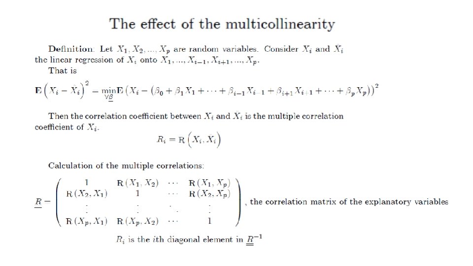
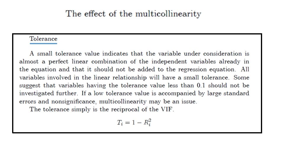
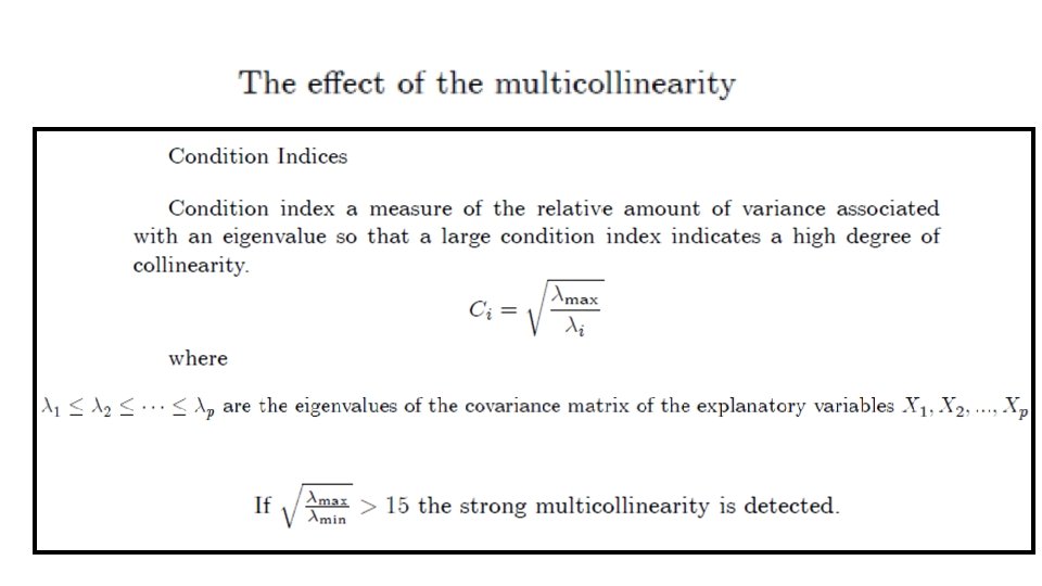
In the case of multicollinearity • the effect of the explanatory variables on the dependent variables can not be separated, • the explanatory variables can assume each other's role, • the estimation of regression coefficients becomes unreliable, • In extreme cases, analysis can not be performed.

Geometrical interpretation of the multiple correlation coefficient. The multiple correlation between the u vector and the pair (x, y) is the cosine of b. This is the angle between u and its projection vector Onto plane spanned by x and y vectors.

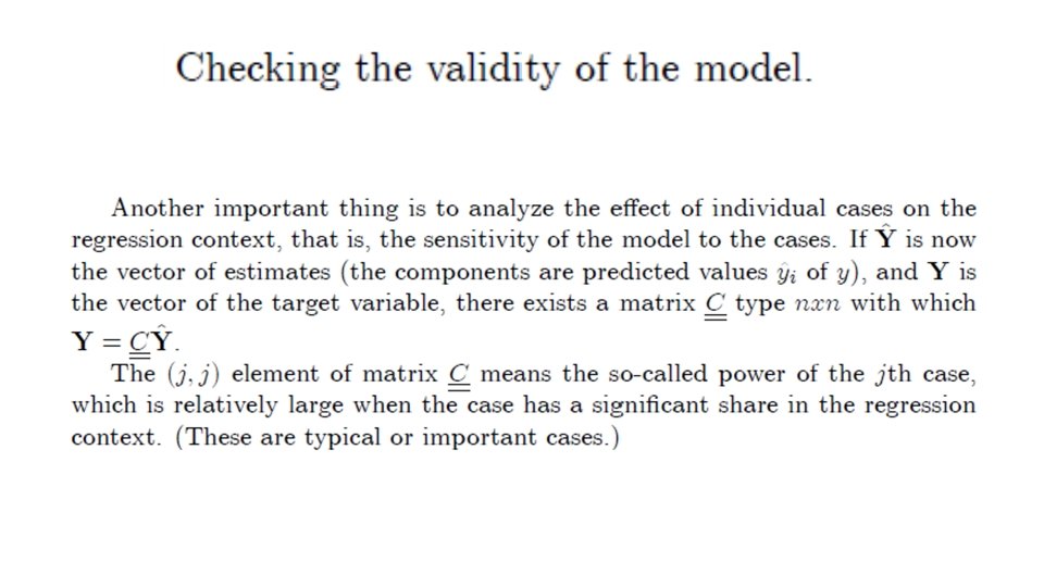
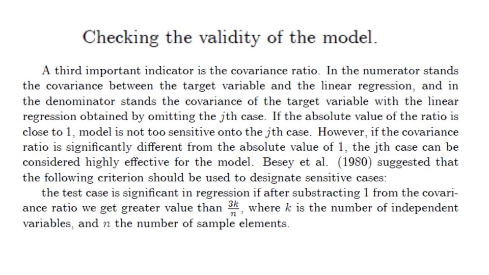
Exploring of the points which effect significantly to the regression An important step in the evaluation of the linear regression model is the exploration of the importance of individual data points. What are the data points that show the ultimate connection most strongly, and what are the so-called outlier points that are least suited to the particular regression context.

Exploring of the points which effect significantly to the regression

Exploring of the points which effect significantly to the regression Connection between the target variable Y and it's linear estimate: Estimated error vector, residual amount, regression amount:

Exploring of the points which effect significantly to the regression the leverage matrix The hii diagonal element of the matrix indicates the quantity of the influence of the i-th data point onto the regression estimation. where the ith data point

Exploring of the points which effect significantly to the regression The influence of case i is average if The influence of case i is significant if Case i can be included in the analysis if It is risky to involve the case i if Case i must be omitted from the analysis because it is "outlier" They are the typical points

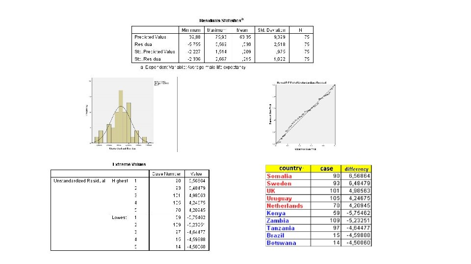
EXAMPLE What and how does it affect life expectancy? Using a data file containing countries, we look for contact between the life expectancy of male and certain economic / social status variables. The dependent variable Y is now the lifeexpm, ie the life expectancy of male The explanatory variables: population density, degree of urbanization, calorie uptake, GDP, yield, child mortality, readership level, birth rate, death rate, population growth, number of children per family.

Y

The automated modeling setup was FORWARD, which takes new variables from the list of variables until it can fix it. It has taken three variables in final: infant mortality, death rate, daily calorie intake.

With the help of the three variables, a 97% explanatory power could be achieved.

The first two variables have negative, the calorie has positive coefficient.

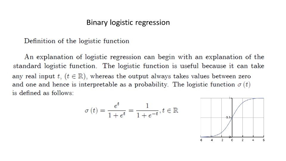
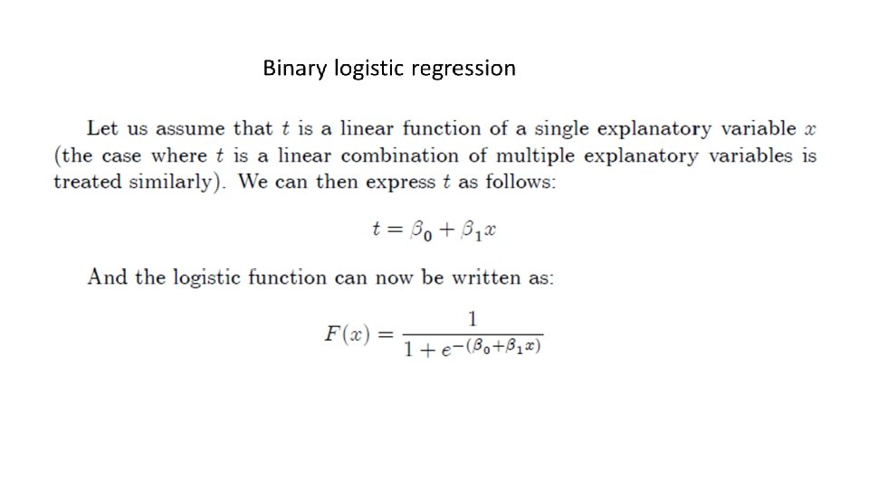
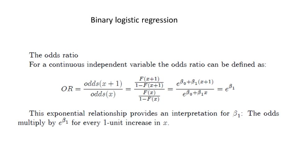
Binary logistic regression

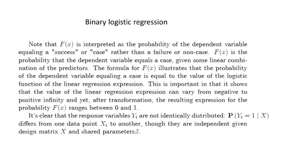
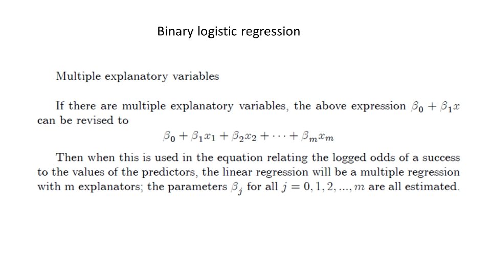
Binary logistic regression

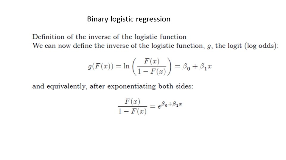
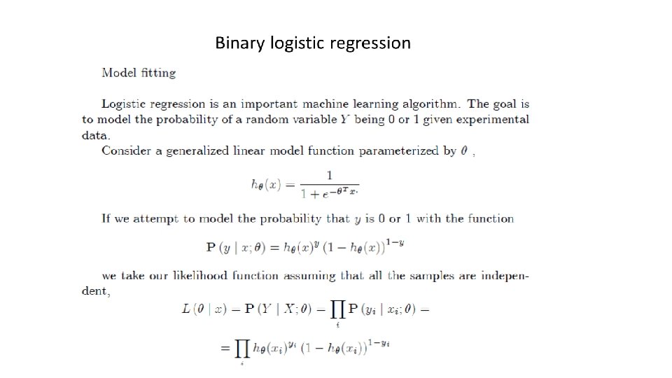
Binary logistic regression

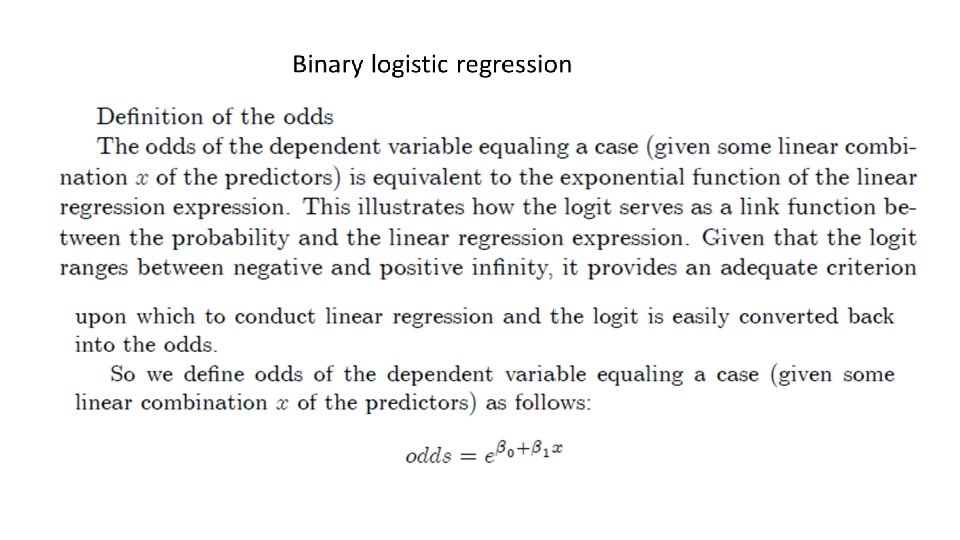
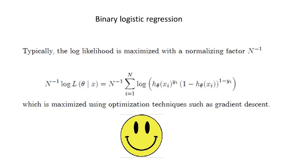
Binary logistic regression

Binary logistic regression