Simple Linear Regression 1 Simple Linear Regression Model

Simple Linear Regression 1

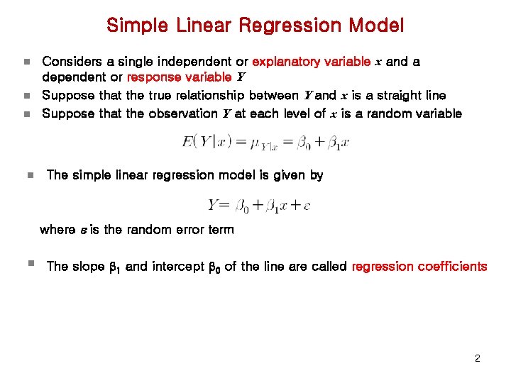
Simple Linear Regression Model n n Considers a single independent or explanatory variable x and a dependent or response variable Y Suppose that the true relationship between Y and x is a straight line Suppose that the observation Y at each level of x is a random variable The simple linear regression model is given by where e is the random error term § The slope b 1 and intercept b 0 of the line are called regression coefficients 2

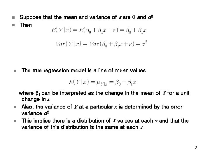
n n n Suppose that the mean and variance of e are 0 and 2 Then The true regression model is a line of mean values where b 1 can be interpreted as the change in the mean of Y for a unit change in x Also, the variance of Y at a particular x is determined by the error variance 2 This implies there is a distribution of Y values at each x and that the variance of this distribution is the same at each x 3

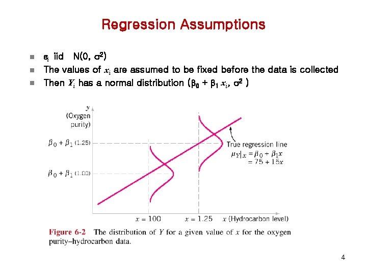
Regression Assumptions n n n i iid N(0, 2) The values of xi are assumed to be fixed before the data is collected Then Yi has a normal distribution (b 0 + b 1 xi, 2 ) 4

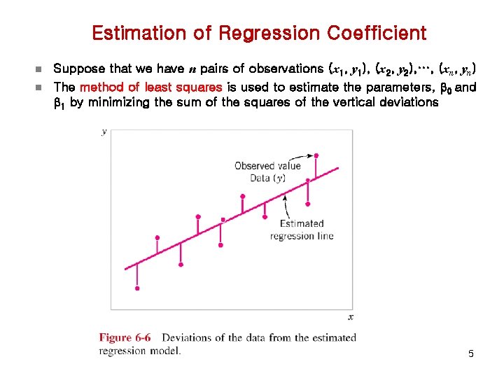
Estimation of Regression Coefficient n n Suppose that we have n pairs of observations (x 1, y 1), (x 2, y 2), …, (xn, yn) The method of least squares is used to estimate the parameters, b 0 and b 1 by minimizing the sum of the squares of the vertical deviations 5

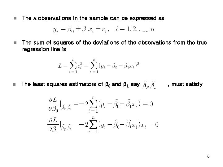
n The n observations in the sample can be expressed as n The sum of squares of the deviations of the observations from the true regression line is n The least squares estimators of b 0 and b 1, say , must satisfy 6

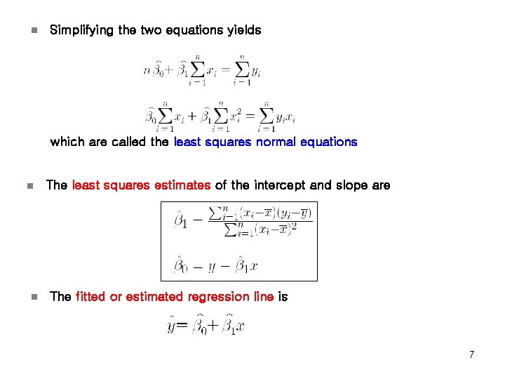
n Simplifying the two equations yields which are called the least squares normal equations n n The least squares estimates of the intercept and slope are The fitted or estimated regression line is 7

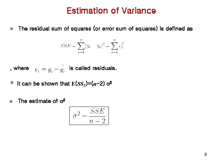
Estimation of Variance n The residual sum of squares (or error sum of squares) is defined as , where is called residuals. § It can be shown that E(SSE)=(n-2) 2 n The estimate of 2 8

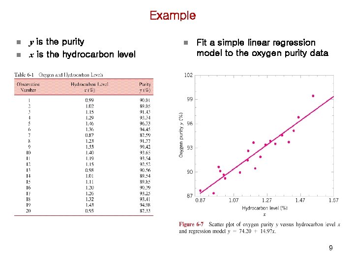
Example n n y is the purity x is the hydrocarbon level n Fit a simple linear regression model to the oxygen purity data 9

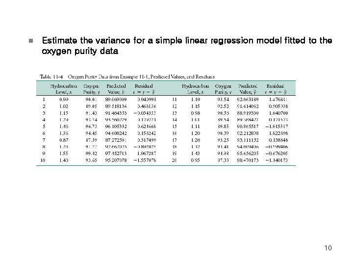
n Estimate the variance for a simple linear regression model fitted to the oxygen purity data 10

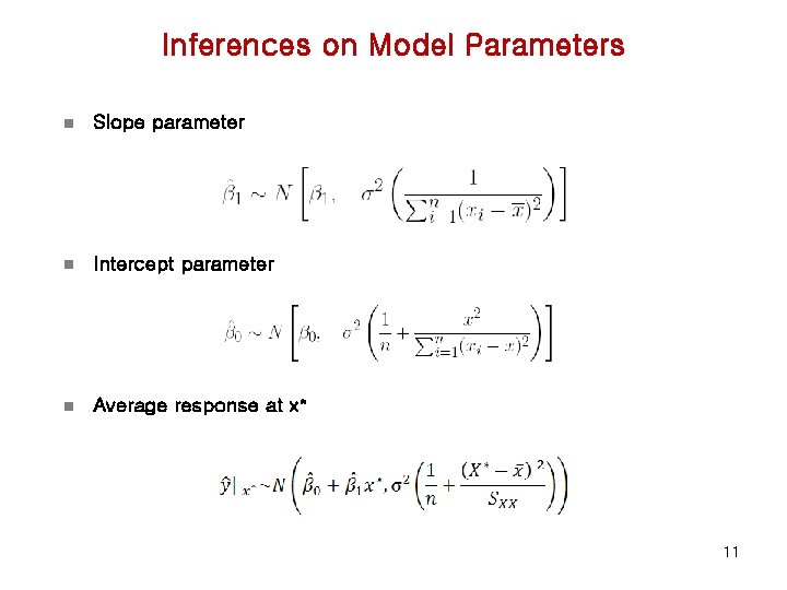
Inferences on Model Parameters n Slope parameter n Intercept parameter n Average response at x* 11

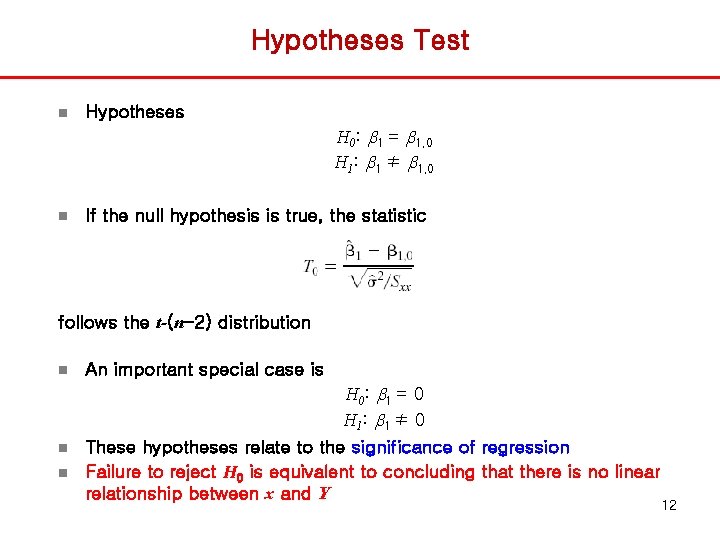
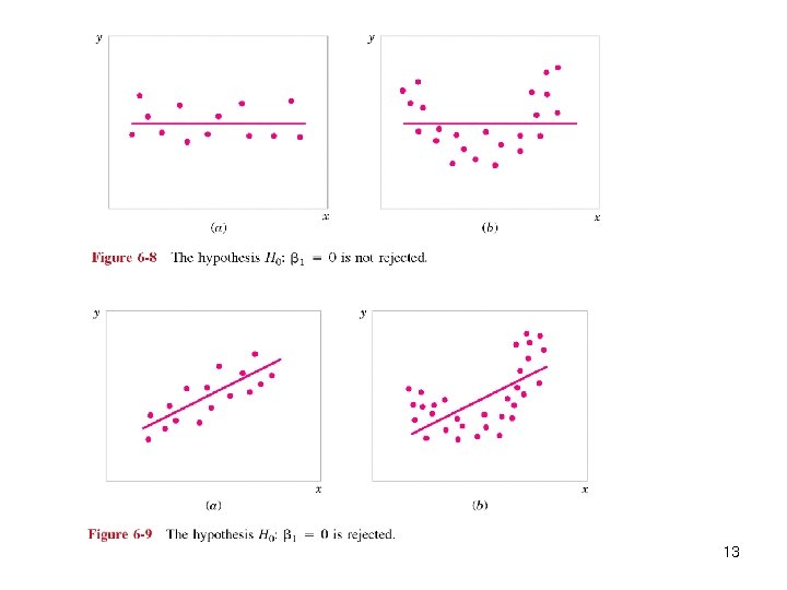
Hypotheses Test n Hypotheses H 0: b 1 = b 1, 0 H 1: b 1 ≠ b 1, 0 n If the null hypothesis is true, the statistic follows the t-(n-2) distribution n An important special case is H 0 : b 1 = 0 H 1 : b 1 ≠ 0 n n These hypotheses relate to the significance of regression Failure to reject H 0 is equivalent to concluding that there is no linear relationship between x and Y 12

13

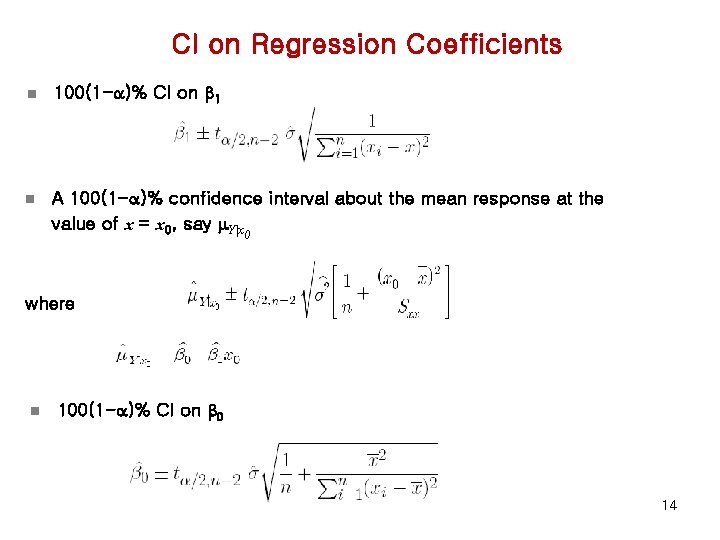
CI on Regression Coefficients n 100(1 -a)% CI on b 1 n A 100(1 -a)% confidence interval about the mean response at the value of x = x 0, say m. Y|x 0 where n 100(1 -a)% CI on b 0 14

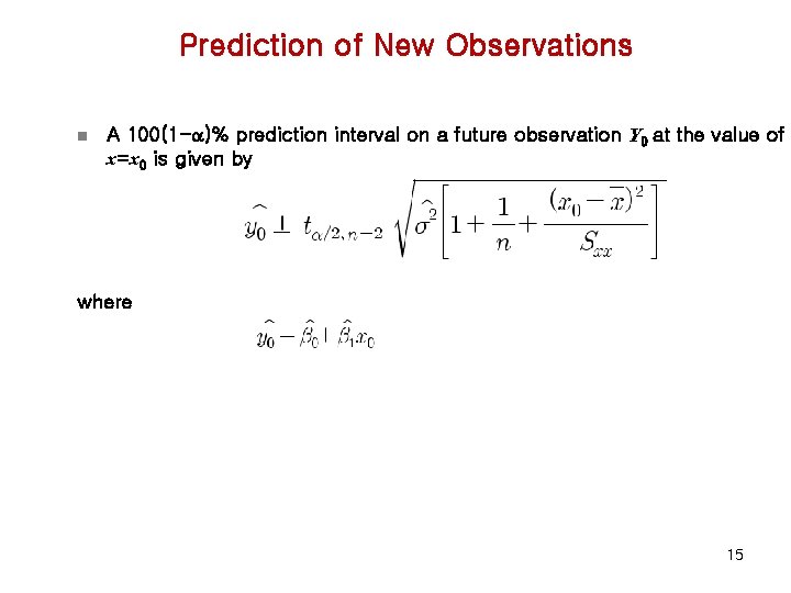
Prediction of New Observations n A 100(1 -a)% prediction interval on a future observation Y 0 at the value of x=x 0 is given by where 15

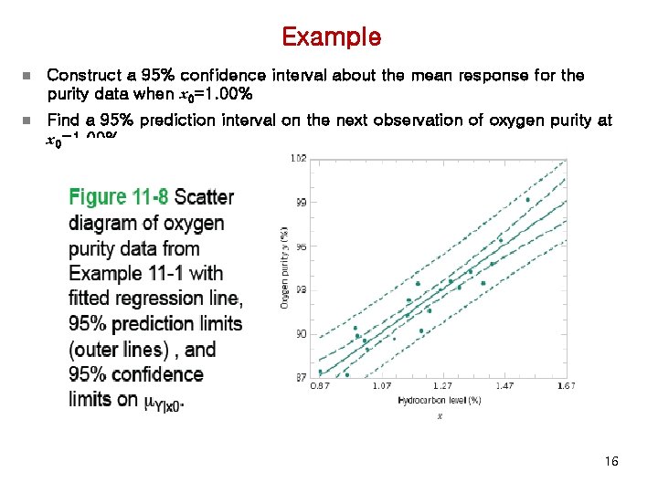
Example n Construct a 95% confidence interval about the mean response for the purity data when x 0=1. 00% n Find a 95% prediction interval on the next observation of oxygen purity at x 0=1. 00% 16

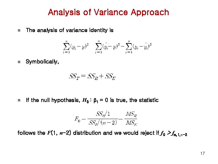
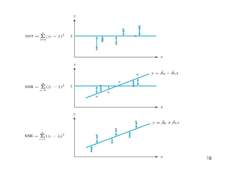
Analysis of Variance Approach n The analysis of variance identity is n Symbolically, n If the null hypothesis, H 0 : b 1 = 0 is true, the statistic follows the F(1, n-2) distribution and we would reject if f 0 > fa, 1, n-2 17

18

19

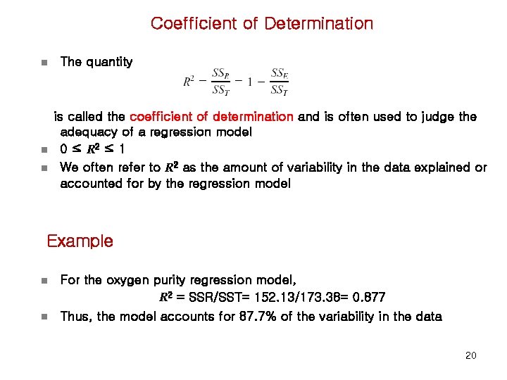
Coefficient of Determination n The quantity is called the coefficient of determination and is often used to judge the adequacy of a regression model 0 ≤ R 2 ≤ 1 We often refer to R 2 as the amount of variability in the data explained or accounted for by the regression model Example n For the oxygen purity regression model, R 2 = SSR/SST= 152. 13/173. 38= 0. 877 n Thus, the model accounts for 87. 7% of the variability in the data 20

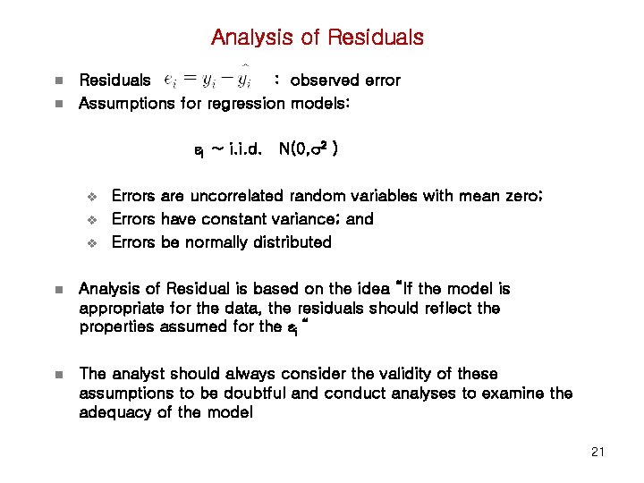
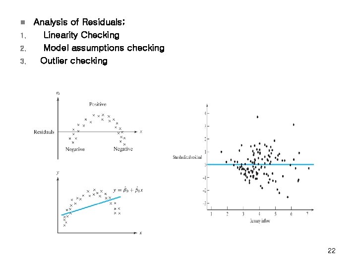
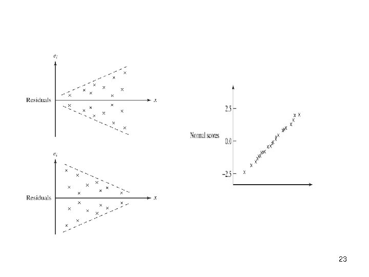
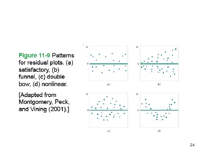
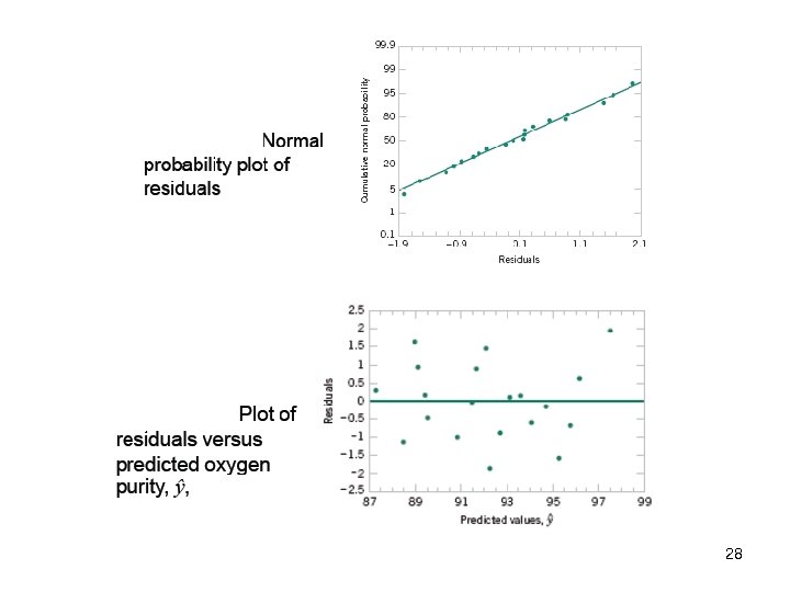
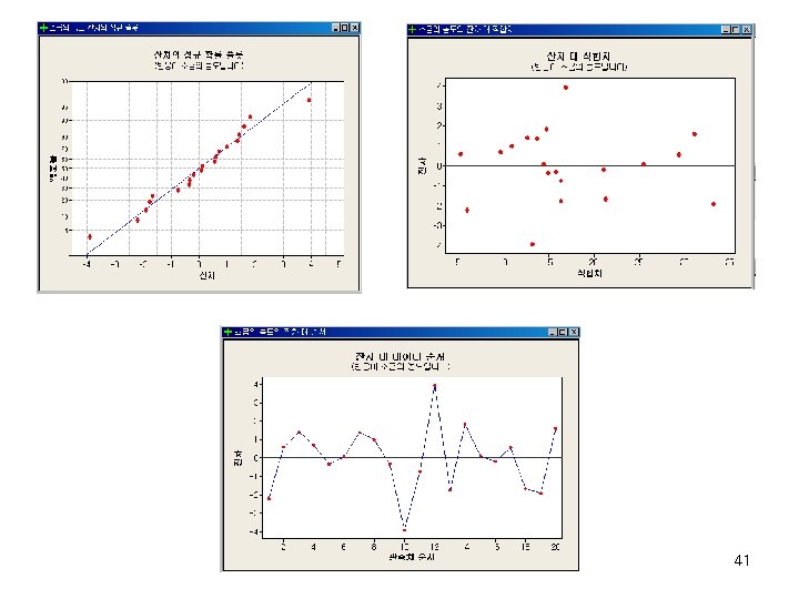
Analysis of Residuals n n Residuals : observed error Assumptions for regression models: I ~ i. i. d. N(0, 2 ) v v v Errors are uncorrelated random variables with mean zero; Errors have constant variance; and Errors be normally distributed n Analysis of Residual is based on the idea “If the model is appropriate for the data, the residuals should reflect the properties assumed for the i “ n The analyst should always consider the validity of these assumptions to be doubtful and conduct analyses to examine the adequacy of the model 21

n 1. 2. 3. Analysis of Residuals; Linearity Checking Model assumptions checking Outlier checking 22

23

24

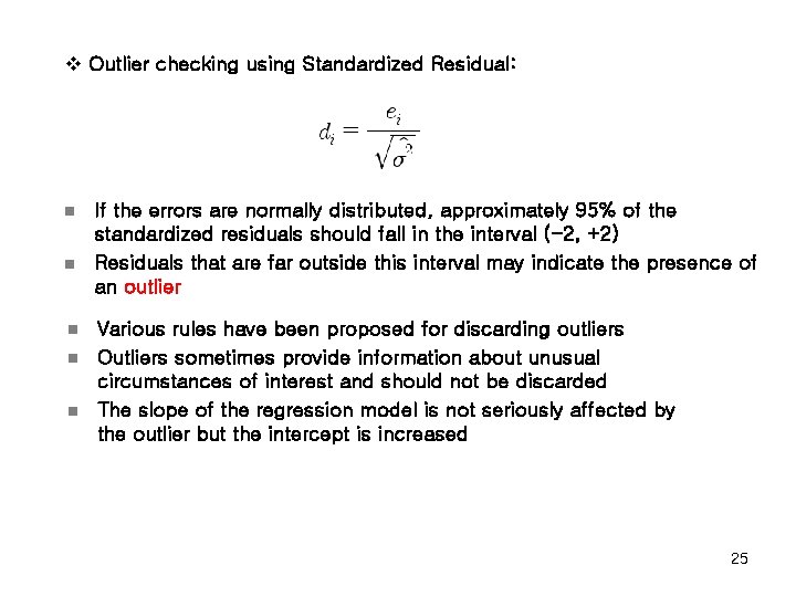
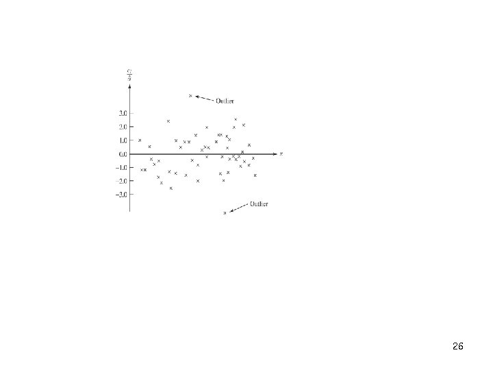
v Outlier checking using Standardized Residual: n n n If the errors are normally distributed, approximately 95% of the standardized residuals should fall in the interval (-2, +2) Residuals that are far outside this interval may indicate the presence of an outlier Various rules have been proposed for discarding outliers Outliers sometimes provide information about unusual circumstances of interest and should not be discarded The slope of the regression model is not seriously affected by the outlier but the intercept is increased 25

26

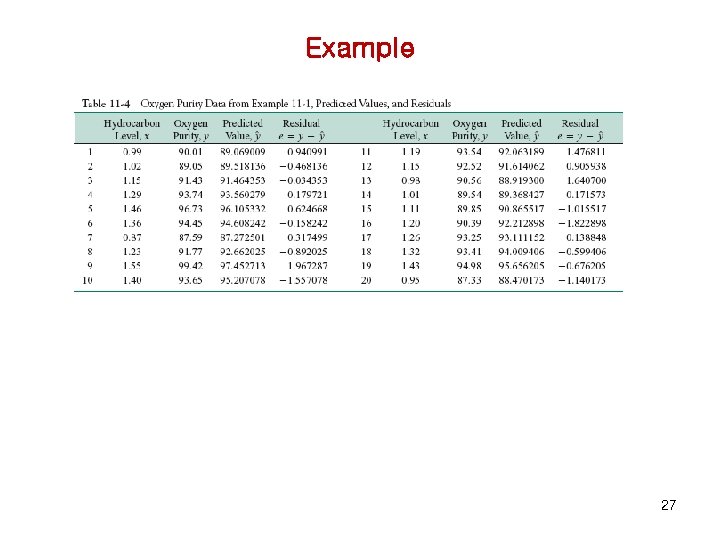
Example 27

28

Correlation & Regression n Correlation is a statistical method used to determine if a linear relationship between variables exists n Regression is the statistical method used to describe the nature of the relationship between variables, that is, positive or negative, linear or nonlinear 29

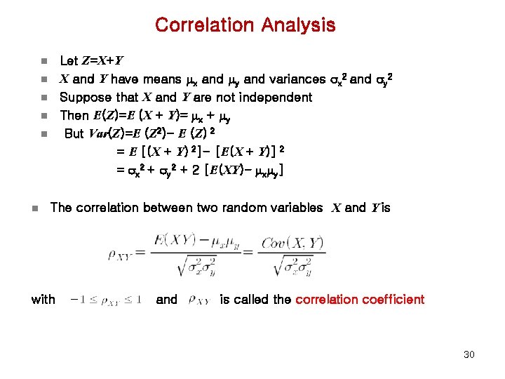
Correlation Analysis Let Z=X+Y X and Y have means mx and my and variances x 2 and y 2 Suppose that X and Y are not independent Then E(Z)=E (X + Y)= mx + my But Var(Z)=E (Z 2)- E (Z) 2 = E [(X + Y) 2]- [E(X + Y)] 2 = x 2 + y 2 + 2 [E(XY)- mxmy] n n n The correlation between two random variables X and Y is with and is called the correlation coefficient 30

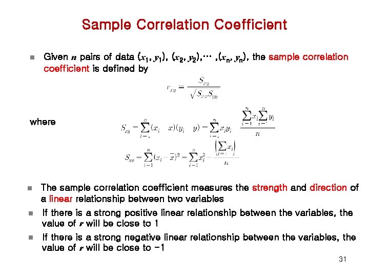
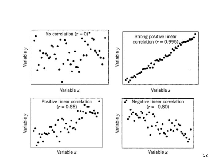
Sample Correlation Coefficient n Given n pairs of data (x 1, y 1), (x 2, y 2), … , (xn, yn), the sample correlation coefficient is defined by where n The sample correlation coefficient measures the strength and direction of a linear relationship between two variables n If there is a strong positive linear relationship between the variables, the value of r will be close to 1 n If there is a strong negative linear relationship between the variables, the value of r will be close to -1 31

32

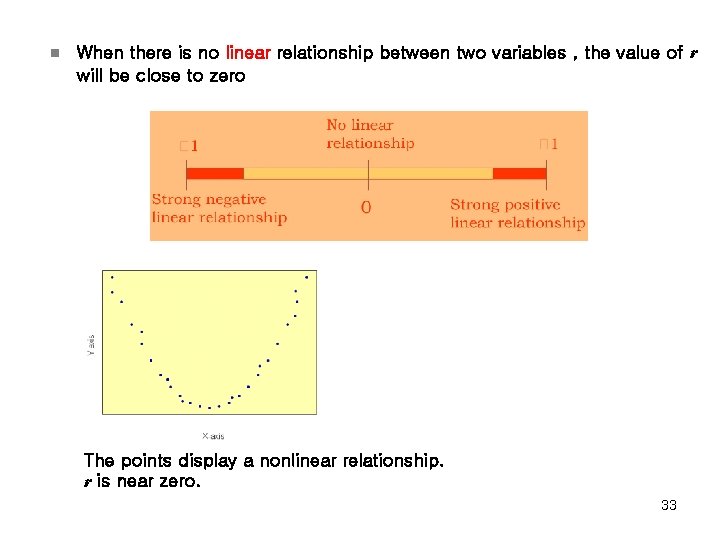
n When there is no linear relationship between two variables , the value of r will be close to zero The points display a nonlinear relationship. r is near zero. 33

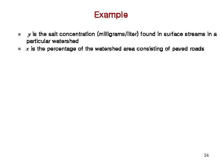
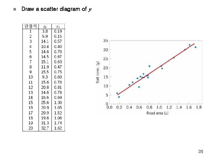
Example n n y is the salt concentration (milligrams/liter) found in surface streams in a particular watershed x is the percentage of the watershed area consisting of paved roads 34

n Draw a scatter diagram of y 35

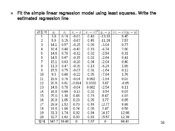
n Fit the simple linear regression model using least squares. Write the estimated regression line 36

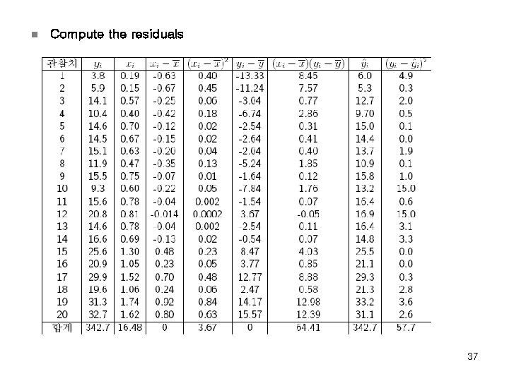
n Compute the residuals 37

n Find an estimate of 2 n Find the standard error of the slope and intercept coefficients n Compute the coefficient of determination. Comment on the value n Use a t test to test for significance of the intercept and slope coefficients at a=0. 05. Comment on your results 38

n Construct the ANOVA table and test for significance of regression n Construct 95% Confidence intervals on the intercept and slope n Compute the sample correlation coefficient and test for its significance at a=0. 05 39

n Construct a 95% confidence interval about the mean salt concentration when roadway area 1. 25% n Construct a 95% prediction interval on a future observation of salt concentration when roadway area 1. 25% n Perform model adequacy checks. Do you believe the model provides an adequate fit? 40

41