Chapter 12 a Simple Linear Regression Simple Linear

Chapter 12 a Simple Linear Regression • • Simple Linear Regression Model Least Squares Method Coefficient of Determination Model Assumptions

Regression may be the most widely used statistical technique in the social and natural sciences—as well as in business

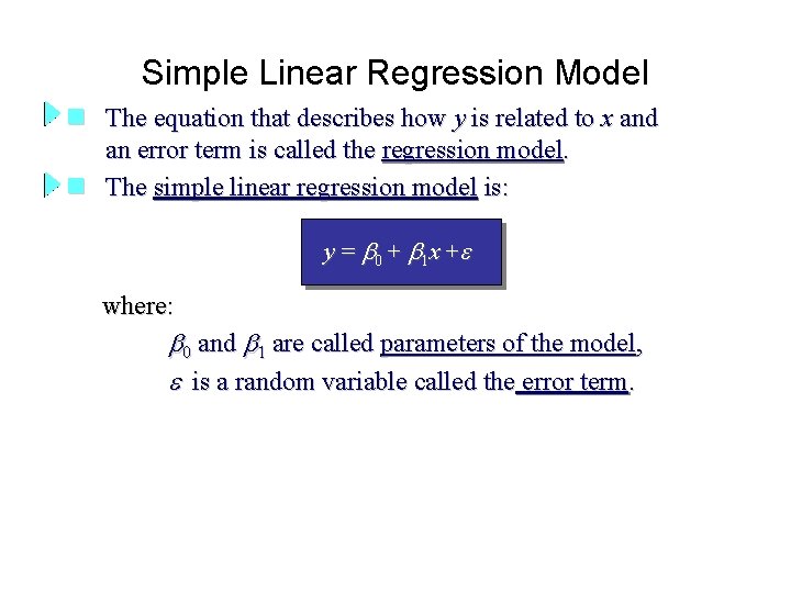
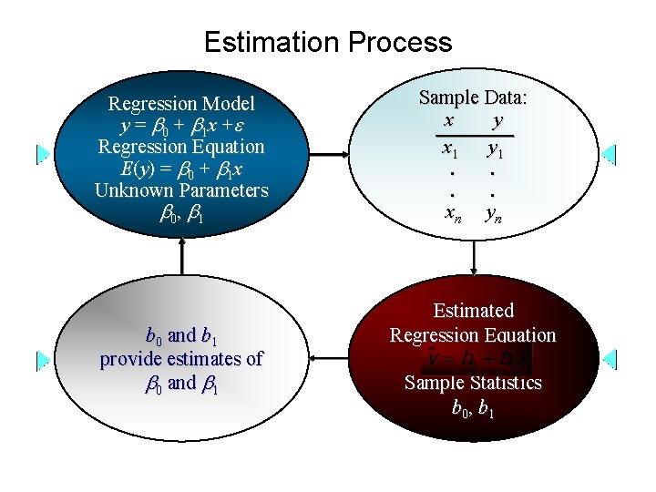
Simple Linear Regression Model n The equation that describes how y is related to x and an error term is called the regression model. n The simple linear regression model is: y = 0 + 1 x + where: 0 and 1 are called parameters of the model, is a random variable called the error term.

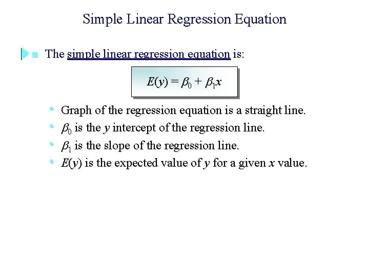
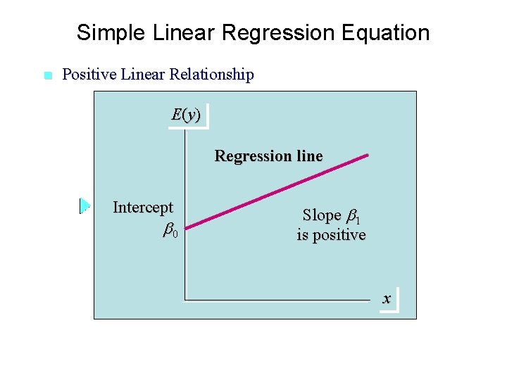
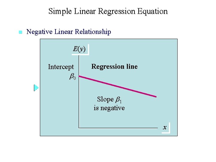
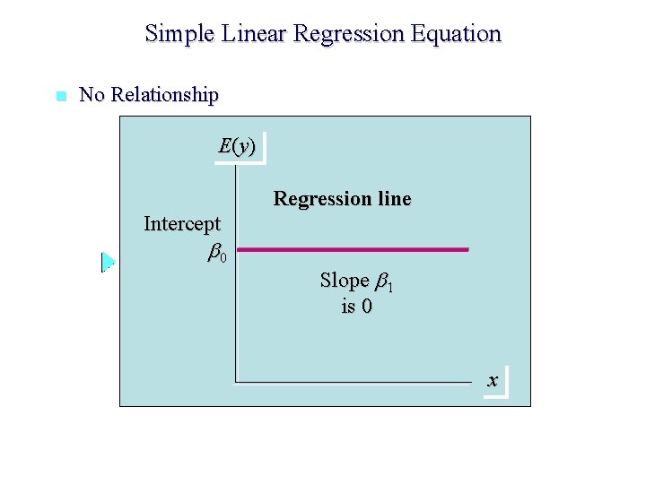
Simple Linear Regression Equation n The simple linear regression equation is: E ( y ) = 0 + 1 x • Graph of the regression equation is a straight line. • 0 is the y intercept of the regression line. • 1 is the slope of the regression line. • E(y) is the expected value of y for a given x value.

Simple Linear Regression Equation n Positive Linear Relationship E (y ) Regression line Intercept 0 Slope 1 is positive x

Simple Linear Regression Equation n Negative Linear Relationship E (y ) Intercept 0 Regression line Slope 1 is negative x

Simple Linear Regression Equation n No Relationship E (y ) Regression line Intercept 0 Slope 1 is 0 x

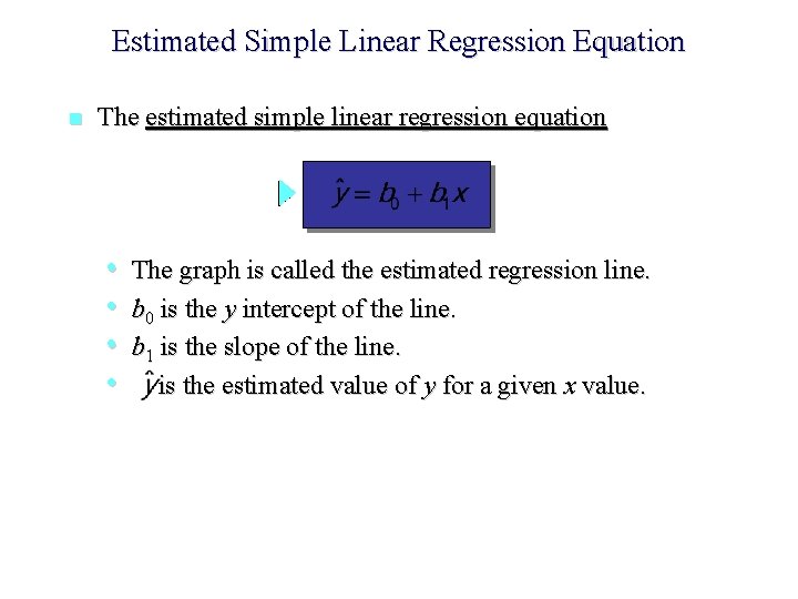
Estimated Simple Linear Regression Equation n The estimated simple linear regression equation • • The graph is called the estimated regression line. b 0 is the y intercept of the line. b 1 is the slope of the line. is the estimated value of y for a given x value.

Estimation Process Regression Model y = 0 + 1 x + Regression Equation E(y) = 0 + 1 x Unknown Parameters 0, 1 b 0 and b 1 provide estimates of 0 and 1 Sample Data: x y x 1 y 1. . xn yn Estimated Regression Equation Sample Statistics b 0, b 1

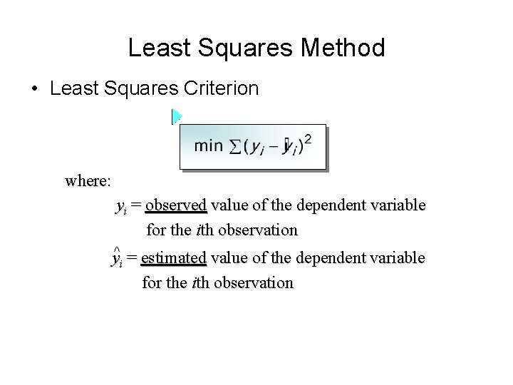
Least Squares Method • Least Squares Criterion where: yi = observed value of the dependent variable for the ith observation y^i = estimated value of the dependent variable for the ith observation

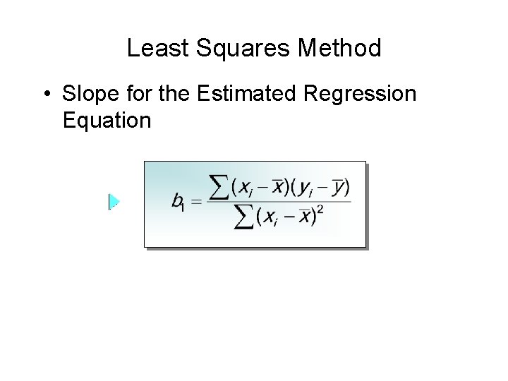
Least Squares Method • Slope for the Estimated Regression Equation

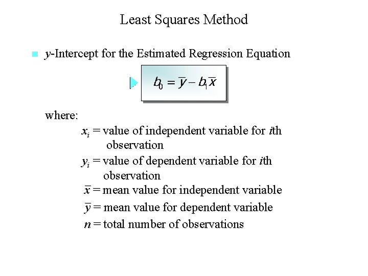
Least Squares Method n y-Intercept for the Estimated Regression Equation where: xi = value of independent variable for ith observation yi = value of dependent variable for ith _ observation x = mean value for independent variable _ y = mean value for dependent variable n = total number of observations

Example: Reed Auto Sales • Simple Linear Regression Reed Auto periodically has a special week-long sale. As part of the advertising campaign Reed runs one or more television commercials during the weekend preceding the sale. Data from a sample of 5 previous sales are shown on the next slide.

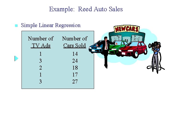
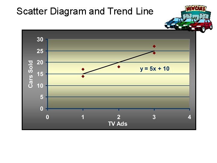
Example: Reed Auto Sales n Simple Linear Regression Number of TV Ads 1 3 2 1 3 Number of Cars Sold 14 24 18 17 27

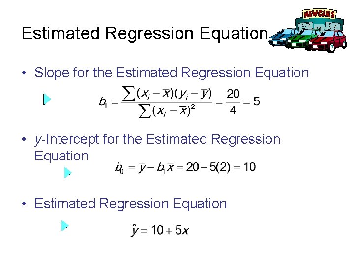
Estimated Regression Equation • Slope for the Estimated Regression Equation • y-Intercept for the Estimated Regression Equation • Estimated Regression Equation

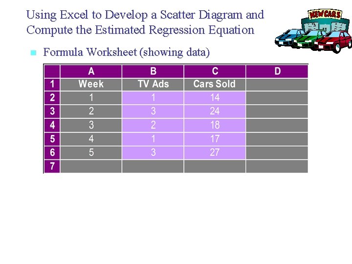
Using Excel to Develop a Scatter Diagram and Compute the Estimated Regression Equation n Formula Worksheet (showing data)

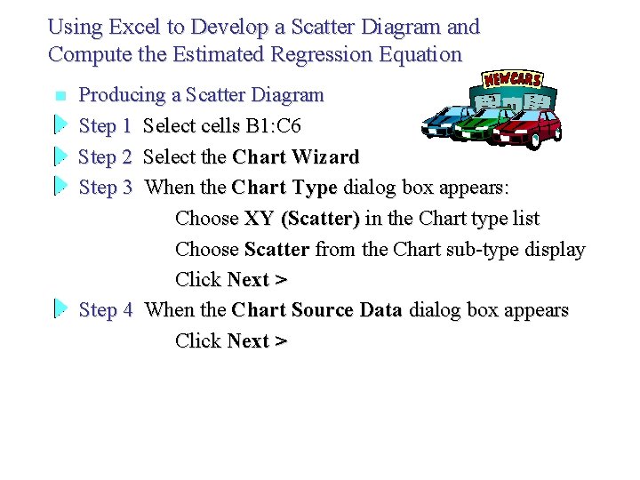
Using Excel to Develop a Scatter Diagram and Compute the Estimated Regression Equation n Producing a Scatter Diagram Step 1 Select cells B 1: C 6 Step 2 Select the Chart Wizard Step 3 When the Chart Type dialog box appears: Choose XY (Scatter) in the Chart type list Choose Scatter from the Chart sub-type display Click Next > Step 4 When the Chart Source Data dialog box appears Click Next >

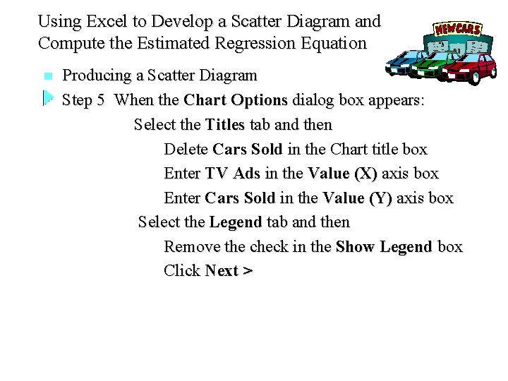
Using Excel to Develop a Scatter Diagram and Compute the Estimated Regression Equation n Producing a Scatter Diagram Step 5 When the Chart Options dialog box appears: Select the Titles tab and then Delete Cars Sold in the Chart title box Enter TV Ads in the Value (X) axis box Enter Cars Sold in the Value (Y) axis box Select the Legend tab and then Remove the check in the Show Legend box Click Next >

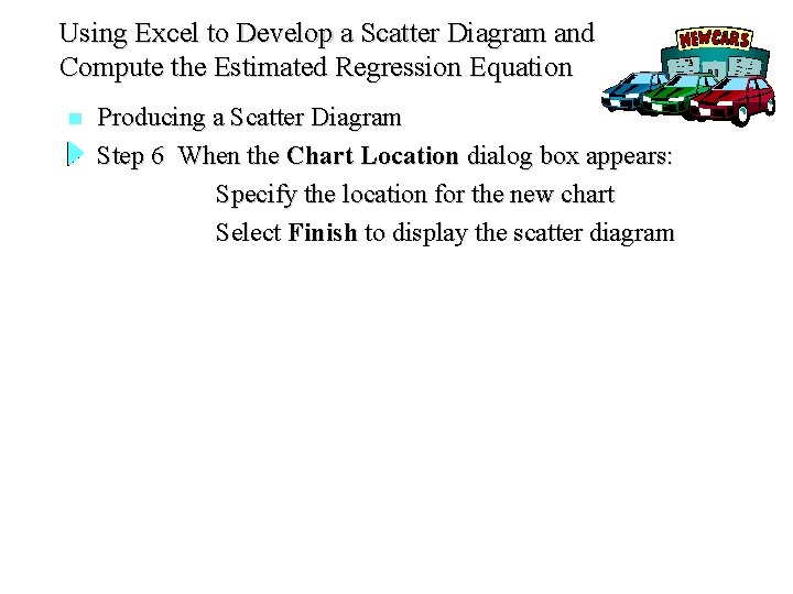
Using Excel to Develop a Scatter Diagram and Compute the Estimated Regression Equation n Producing a Scatter Diagram Step 6 When the Chart Location dialog box appears: Specify the location for the new chart Select Finish to display the scatter diagram

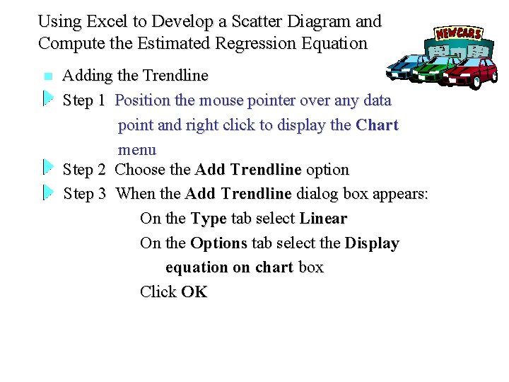
Using Excel to Develop a Scatter Diagram and Compute the Estimated Regression Equation n Adding the Trendline Step 1 Position the mouse pointer over any data point and right click to display the Chart menu Step 2 Choose the Add Trendline option Step 3 When the Add Trendline dialog box appears: On the Type tab select Linear On the Options tab select the Display equation on chart box Click OK

Scatter Diagram and Trend Line

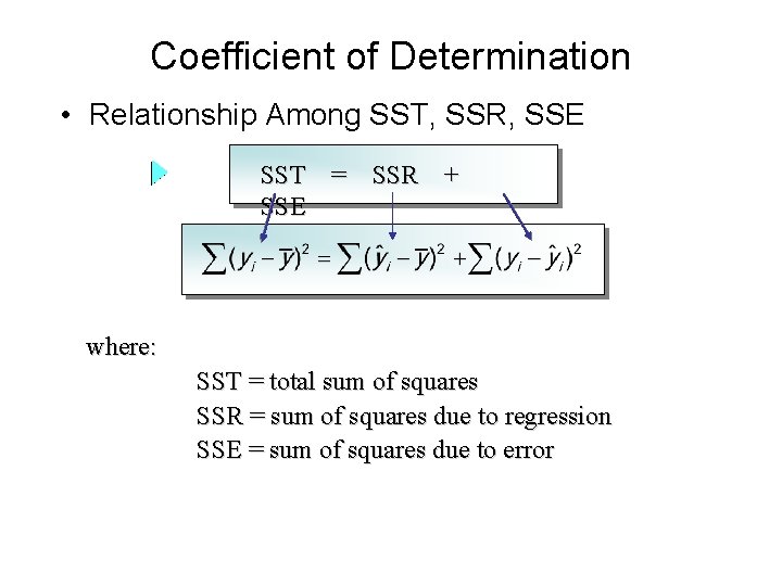
Coefficient of Determination • Relationship Among SST, SSR, SSE SST = SSR + SSE where: SST = total sum of squares SSR = sum of squares due to regression SSE = sum of squares due to error

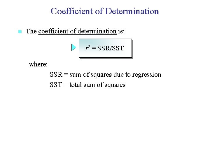
Coefficient of Determination n The coefficient of determination is: r 2 = SSR/SST where: SSR = sum of squares due to regression SST = total sum of squares

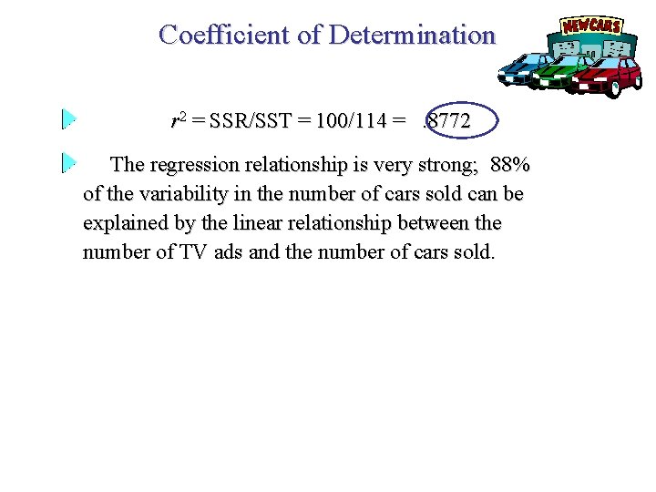
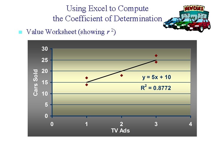
Coefficient of Determination r 2 = SSR/SST = 100/114 =. 8772 The regression relationship is very strong; 88% of the variability in the number of cars sold can be explained by the linear relationship between the number of TV ads and the number of cars sold.

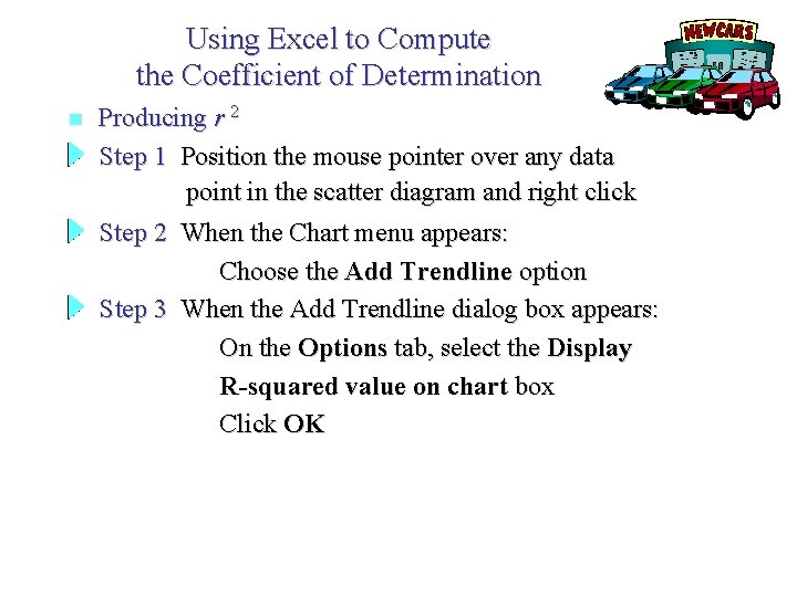
Using Excel to Compute the Coefficient of Determination n Producing r 2 Step 1 Position the mouse pointer over any data point in the scatter diagram and right click Step 2 When the Chart menu appears: Choose the Add Trendline option Step 3 When the Add Trendline dialog box appears: On the Options tab, select the Display R-squared value on chart box Click OK

Using Excel to Compute the Coefficient of Determination n Value Worksheet (showing r 2)

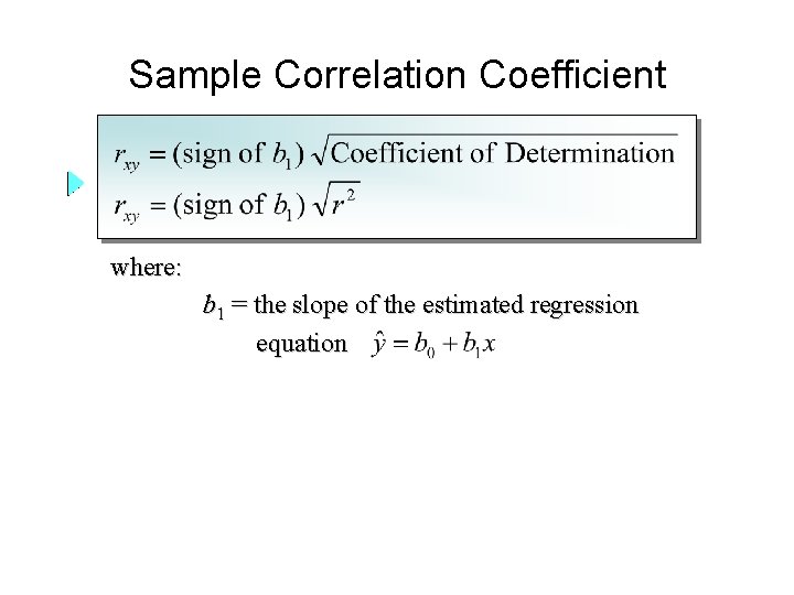
Sample Correlation Coefficient where: b 1 = the slope of the estimated regression equation

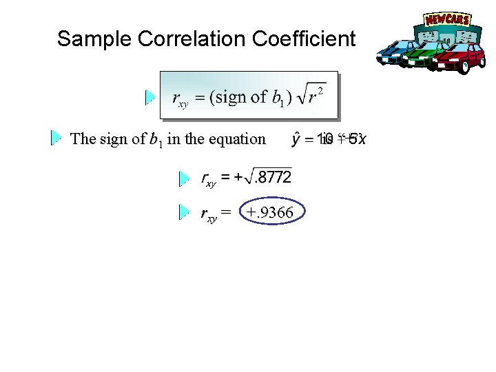
Sample Correlation Coefficient The sign of b 1 in the equation rxy = +. 9366 is “+”.

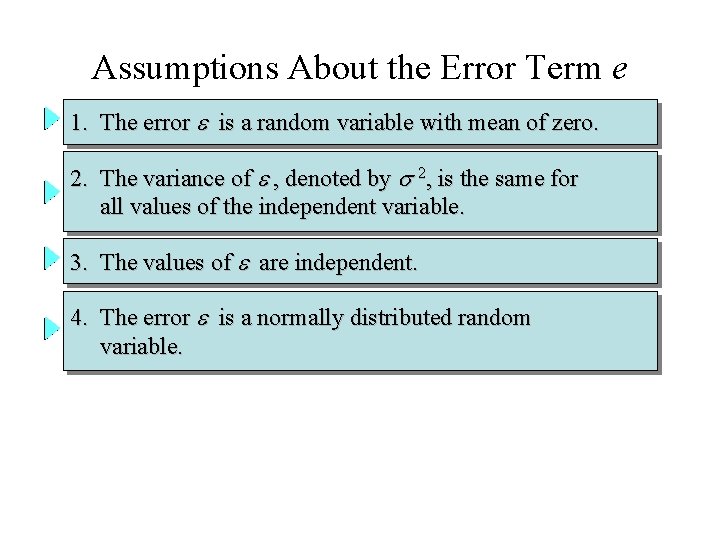
Assumptions About the Error Term e 1. The error is a random variable with mean of zero. 2. The variance of , denoted by 2, is the same for all values of the independent variable. 3. The values of are independent. 4. The error is a normally distributed random variable.