12 Simple Linear Regression and Correlation Copyright Cengage

12 Simple Linear Regression and Correlation Copyright © Cengage Learning. All rights reserved.

12. 3 Inferences About the Slope Parameter 1 Copyright © Cengage Learning. All rights reserved.

Inferences About the Slope Parameter 1 In virtually all of our inferential work thus far, the notion of sampling variability has been pervasive. In particular, properties of sampling distributions of various statistics have been the basis for developing confidence interval formulas and hypothesis-testing methods. The key idea here is that the value of any quantity calculated from sample data—the value of any statistic—will vary from one sample to another. 3

Example 10 The following data is representative of that reported in the article “An Experimental Correlation of Oxides of Nitrogen Emissions from Power Boilers Based on Field Data” (J. of Engr. for Power, July 1973: 165– 170), x = burner-area liberation rate (MBtu/hr-ft 2) and y = NOx emission rate (ppm). There are 14 observations, made at the x values 100, 125, 150, 200, 250, 300, 350, 400, and 400, respectively. 4

Example 10 cont’d Suppose that the slope and intercept of the true regression line are 1 = 1. 70 and 0 = – 50, with = 35 (consistent with the values = 1. 7114, = – 45. 55, s = 36. 75). We proceeded to generate a sample of random deviations from a normal distribution with mean 0 and standard deviation 35 and then added to 0 + 1 xi obtain 14 corresponding y values. Regression calculations were then carried out to obtain the estimated slope, intercept, and standard deviation. 5

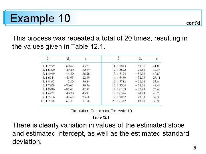
Example 10 cont’d This process was repeated a total of 20 times, resulting in the values given in Table 12. 1. Simulation Results for Example 10 Table 12. 1 There is clearly variation in values of the estimated slope and estimated intercept, as well as the estimated standard deviation. 6

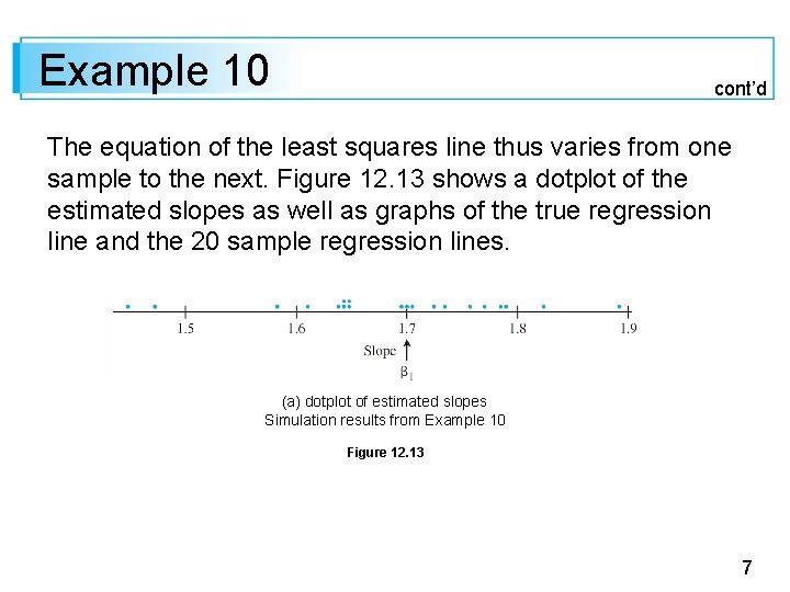
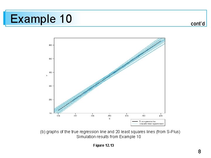
Example 10 cont’d The equation of the least squares line thus varies from one sample to the next. Figure 12. 13 shows a dotplot of the estimated slopes as well as graphs of the true regression line and the 20 sample regression lines. (a) dotplot of estimated slopes Simulation results from Example 10 Figure 12. 13 7

Example 10 cont’d (b) graphs of the true regression line and 20 least squares lines (from S-Plus) Simulation results from Example 10 Figure 12. 13 8

Inferences About the Slope Parameter 1 The slope 1 of the population regression line is the true average change in the dependent variable y associated with a 1 -unit increase in the independent variable x. The slope of the least squares line, , gives a point estimate of 1. In the same way that a confidence interval for and procedures for testing hypotheses about were based on properties of the sampling distribution of , further inferences about 1 are based on thinking of as a statistic and investigating its sampling distribution. The values of the xi’s are assumed to be chosen before the experiment is performed, so only the Yi’s are random. 9

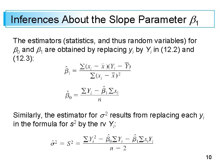
Inferences About the Slope Parameter 1 The estimators (statistics, and thus random variables) for 0 and 1 are obtained by replacing yi by Yi in (12. 2) and (12. 3): Similarly, the estimator for 2 results from replacing each yi in the formula for s 2 by the rv Yi: 10

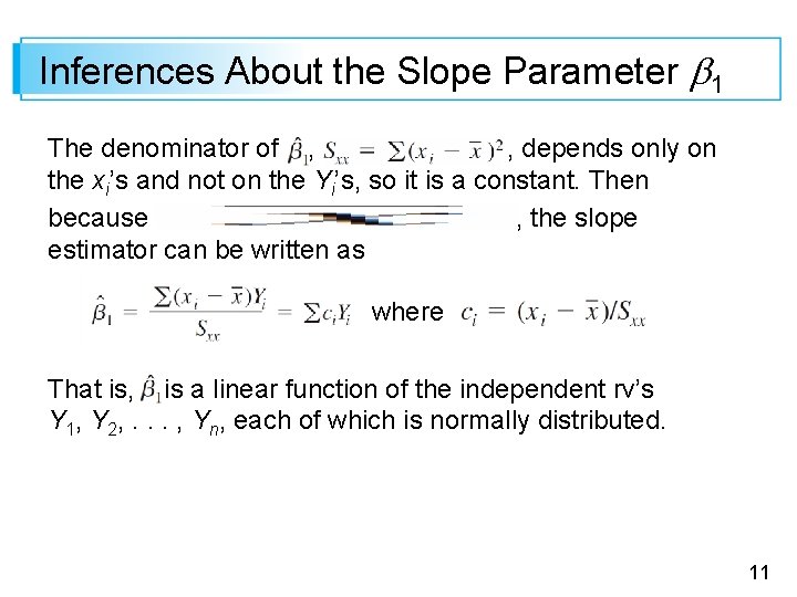
Inferences About the Slope Parameter 1 The denominator of , , depends only on the xi’s and not on the Yi’s, so it is a constant. Then because , the slope estimator can be written as where That is, is a linear function of the independent rv’s Y 1, Y 2, . . . , Yn, each of which is normally distributed. 11

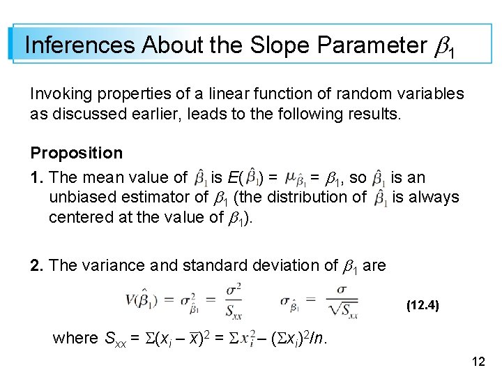
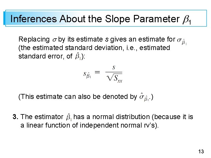
Inferences About the Slope Parameter 1 Invoking properties of a linear function of random variables as discussed earlier, leads to the following results. Proposition 1. The mean value of is E( ) = = 1, so unbiased estimator of 1 (the distribution of centered at the value of 1). is an is always 2. The variance and standard deviation of 1 are (12. 4) where Sxx = (xi – x)2 = – ( xi)2/n. 12

Inferences About the Slope Parameter 1 Replacing by its estimate s gives an estimate for (the estimated standard deviation, i. e. , estimated standard error, of ): (This estimate can also be denoted by . ) 3. The estimator has a normal distribution (because it is a linear function of independent normal rv’s). 13

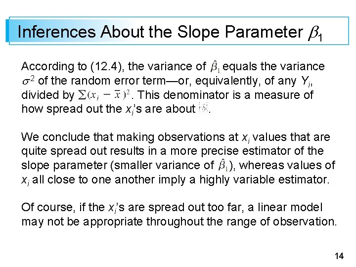
Inferences About the Slope Parameter 1 According to (12. 4), the variance of equals the variance 2 of the random error term—or, equivalently, of any Yi, divided by. This denominator is a measure of how spread out the xi’s are about. We conclude that making observations at xi values that are quite spread out results in a more precise estimator of the slope parameter (smaller variance of ), whereas values of xi all close to one another imply a highly variable estimator. Of course, if the xi’s are spread out too far, a linear model may not be appropriate throughout the range of observation. 14

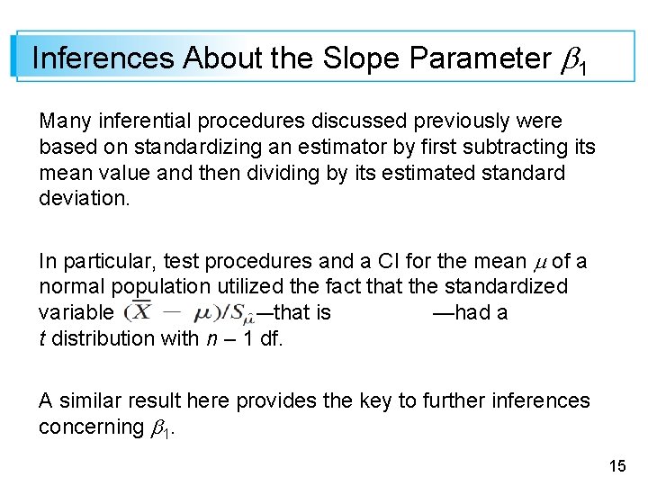
Inferences About the Slope Parameter 1 Many inferential procedures discussed previously were based on standardizing an estimator by first subtracting its mean value and then dividing by its estimated standard deviation. In particular, test procedures and a CI for the mean of a normal population utilized the fact that the standardized variable —that is —had a t distribution with n – 1 df. A similar result here provides the key to further inferences concerning 1. 15

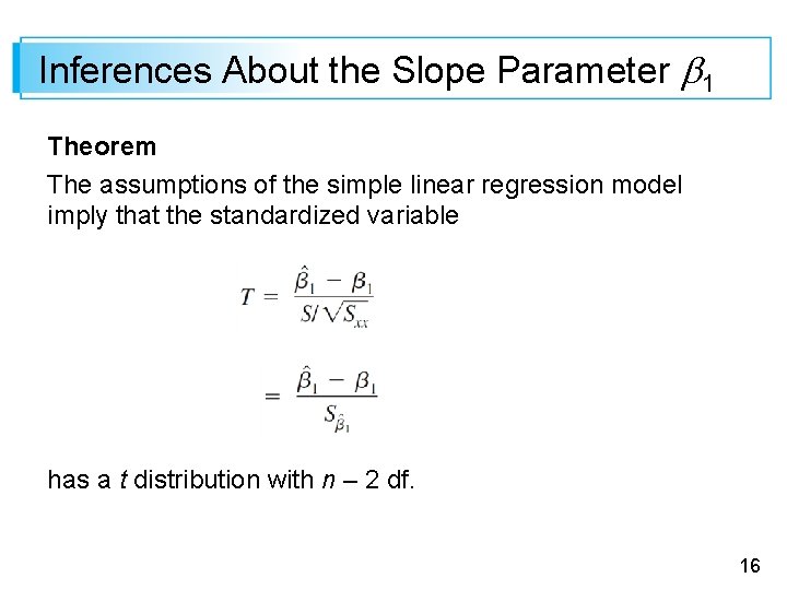
Inferences About the Slope Parameter 1 Theorem The assumptions of the simple linear regression model imply that the standardized variable has a t distribution with n – 2 df. 16

A Confidence Interval for 1 17

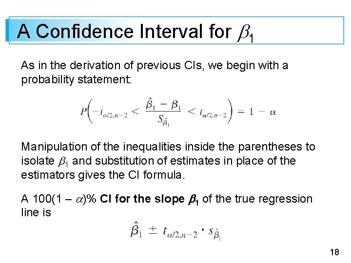
A Confidence Interval for 1 As in the derivation of previous CIs, we begin with a probability statement: Manipulation of the inequalities inside the parentheses to isolate 1 and substitution of estimates in place of the estimators gives the CI formula. A 100(1 – )% CI for the slope 1 of the true regression line is 18

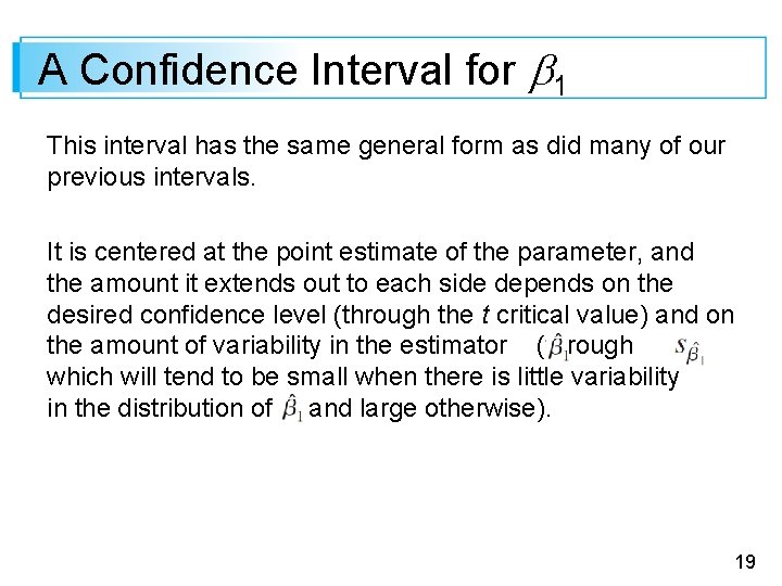
A Confidence Interval for 1 This interval has the same general form as did many of our previous intervals. It is centered at the point estimate of the parameter, and the amount it extends out to each side depends on the desired confidence level (through the t critical value) and on the amount of variability in the estimator (through , which will tend to be small when there is little variability in the distribution of and large otherwise). 19

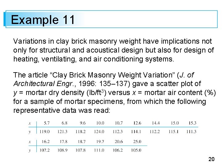
Example 11 Variations in clay brick masonry weight have implications not only for structural and acoustical design but also for design of heating, ventilating, and air conditioning systems. The article “Clay Brick Masonry Weight Variation” (J. of Architectural Engr. , 1996: 135– 137) gave a scatter plot of y = mortar dry density (lb/ft 3) versus x = mortar air content (%) for a sample of mortar specimens, from which the following representative data was read: 20

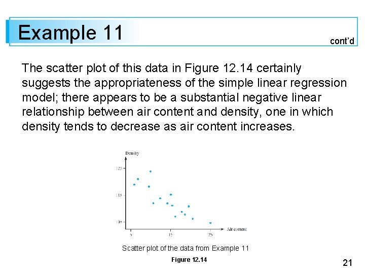
Example 11 cont’d The scatter plot of this data in Figure 12. 14 certainly suggests the appropriateness of the simple linear regression model; there appears to be a substantial negative linear relationship between air content and density, one in which density tends to decrease as air content increases. Scatter plot of the data from Example 11 Figure 12. 14 21

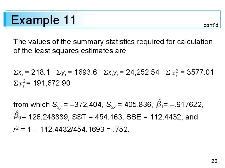
Example 11 cont’d The values of the summary statistics required for calculation of the least squares estimates are xi = 218. 1 yi = 1693. 6 xiyi = 24, 252. 54 = 191, 672. 90 from which Sxy = – 372. 404, Sxx = 405. 836, = 3577. 01 = –. 917622, = 126. 248889, SST = 454. 163, SSE = 112. 4432, and r 2 = 1 – 112. 4432/454. 1693 =. 752. 22

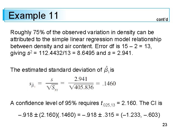
Example 11 cont’d Roughly 75% of the observed variation in density can be attributed to the simple linear regression model relationship between density and air content. Error df is 15 – 2 = 13, giving s 2 = 112. 4432/13 = 8. 6495 and s = 2. 941. The estimated standard deviation of is A confidence level of 95% requires t. 025, 13 = 2. 160. The CI is –. 918 (2. 160)(. 1460) = –. 918 . 315 = (– 1. 233, –. 603) 23

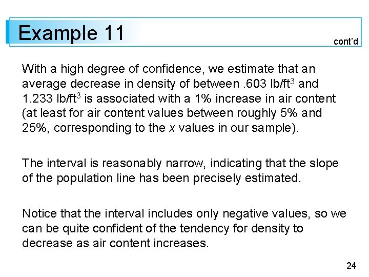
Example 11 cont’d With a high degree of confidence, we estimate that an average decrease in density of between. 603 lb/ft 3 and 1. 233 lb/ft 3 is associated with a 1% increase in air content (at least for air content values between roughly 5% and 25%, corresponding to the x values in our sample). The interval is reasonably narrow, indicating that the slope of the population line has been precisely estimated. Notice that the interval includes only negative values, so we can be quite confident of the tendency for density to decrease as air content increases. 24

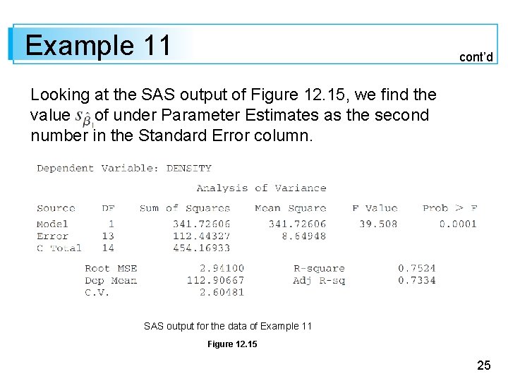
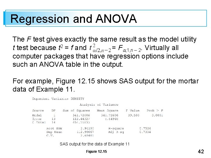
Example 11 cont’d Looking at the SAS output of Figure 12. 15, we find the value of under Parameter Estimates as the second number in the Standard Error column. SAS output for the data of Example 11 Figure 12. 15 25

Example 11 cont’d SAS output for the data of Example 11 Figure 12. 15 26

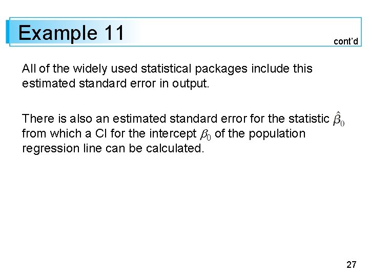
Example 11 cont’d All of the widely used statistical packages include this estimated standard error in output. There is also an estimated standard error for the statistic from which a CI for the intercept 0 of the population regression line can be calculated. 27

Hypothesis-Testing Procedures 28

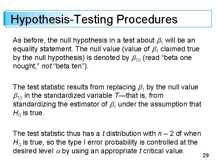
Hypothesis-Testing Procedures As before, the null hypothesis in a test about 1 will be an equality statement. The null value (value of 1 claimed true by the null hypothesis) is denoted by 10 (read “beta one nought, ” not “beta ten”). The test statistic results from replacing 1 by the null value 10 in the standardized variable T—that is, from standardizing the estimator of 1 under the assumption that H 0 is true. The test statistic thus has a t distribution with n – 2 df when H 0 is true, so the type I error probability is controlled at the desired level by using an appropriate t critical value. 29

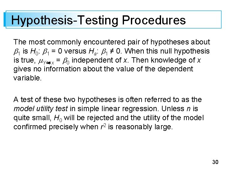
Hypothesis-Testing Procedures The most commonly encountered pair of hypotheses about 1 is H 0: 1 = 0 versus Ha: 1 ≠ 0. When this null hypothesis is true, Y x = 0 independent of x. Then knowledge of x gives no information about the value of the dependent variable. A test of these two hypotheses is often referred to as the model utility test in simple linear regression. Unless n is quite small, H 0 will be rejected and the utility of the model confirmed precisely when r 2 is reasonably large. 30

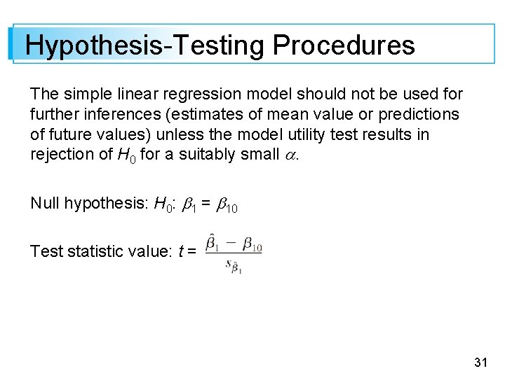
Hypothesis-Testing Procedures The simple linear regression model should not be used for further inferences (estimates of mean value or predictions of future values) unless the model utility test results in rejection of H 0 for a suitably small . Null hypothesis: H 0: 1 = 10 Test statistic value: t = 31

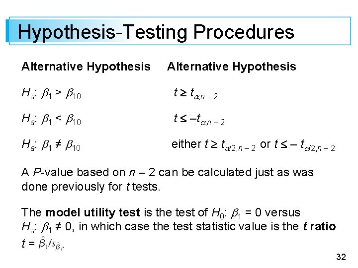
Hypothesis-Testing Procedures Alternative Hypothesis Ha: 1 > 10 t t , n – 2 Ha: 1 < 10 t –t , n – 2 Ha: 1 ≠ 10 either t t /2, n – 2 or t – t /2, n – 2 A P-value based on n – 2 can be calculated just as was done previously for t tests. The model utility test is the test of H 0: 1 = 0 versus Ha: 1 ≠ 0, in which case the test statistic value is the t ratio t=. 32

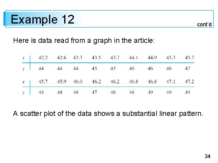
Example 12 Mopeds are very popular in Europe because of cost and ease of operation. However, they can be dangerous if performance characteristics are modified. One of the features commonly manipulated is the maximum speed. The article “Procedure to Verify the Maximum Speed of Automatic Transmission Mopeds in Periodic Motor Vehicle Inspections” (J. of Automotive Engr. , 2008: 1615– 1623) included a simple linear regression analysis of the variables x = test track speed (km/h) and y = rolling test speed. 33

Example 12 cont’d Here is data read from a graph in the article: A scatter plot of the data shows a substantial linear pattern. 34

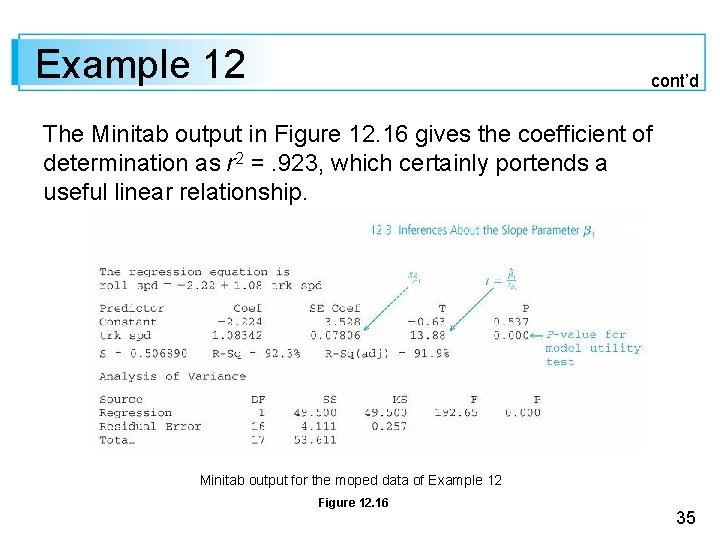
Example 12 cont’d The Minitab output in Figure 12. 16 gives the coefficient of determination as r 2 =. 923, which certainly portends a useful linear relationship. Minitab output for the moped data of Example 12 Figure 12. 16 35

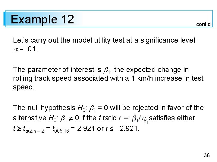
Example 12 cont’d Let’s carry out the model utility test at a significance level =. 01. The parameter of interest is 1, the expected change in rolling track speed associated with a 1 km/h increase in test speed. The null hypothesis H 0: 1 = 0 will be rejected in favor of the alternative H 0: 1 0 if the t ratio satisfies either t t /2, n – 2 = t 005, 16 = 2. 921 or t – 2. 921. 36

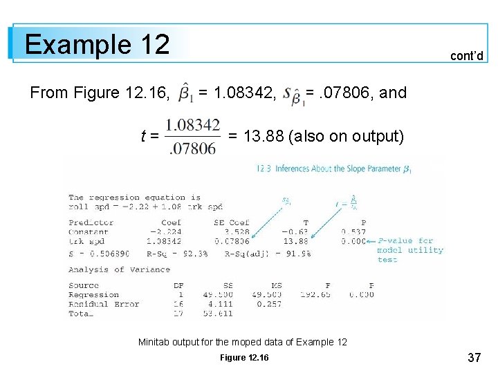
Example 12 From Figure 12. 16, t= cont’d = 1. 08342, =. 07806, and = 13. 88 (also on output) Minitab output for the moped data of Example 12 Figure 12. 16 37

Example 12 cont’d Clearly this t ratio falls well into the upper tail of the two-tailed rejection region, so H 0 is resoundingly rejected. Alternatively, the P-value is twice the area captured under the 16 df t curve to the right of 13. 88. Minitab gives P-value =. 000. Thus the null hypothesis of no useful linear relationship can be rejected at any reasonable significance level. This confirms the utility of the model, and gives us license to calculate various estimates and predictions. 38

Regression and ANOVA 39

Regression and ANOVA The decomposition of the total sum of squares into a part SSE, which measures unexplained variation, and a part SSR, which measures variation explained by the linear relationship, is strongly reminiscent of one-way ANOVA. 40

Regression and ANOVA In fact, the null hypothesis H 0: 1 = 0 can be tested against Ha: 1 0 by constructing an ANOVA table (Table 12. 2) and rejecting H 0 if f F , 1, n – 2. ANOVA Table for Simple Linear Regression Table 12. 2 41

Regression and ANOVA The F test gives exactly the same result as the model utility t test because t 2 = f and = F , 1, n – 2. Virtually all computer packages that have regression options include such an ANOVA table in the output. For example, Figure 12. 15 shows SAS output for the mortar data of Example 11. SAS output for the data of Example 11 Figure 12. 15 42

Regression and ANOVA cont’d SAS output for the data of Example 11 Figure 12. 15 43

Regression and ANOVA The ANOVA table at the top of the output has f = 39. 508 with a P-value of. 0001 for the model utility test. The table of parameter estimates gives t = – 6. 286, again with P =. 0001 and (– 6. 286)2 = 39. 51. 44