Chapter 16 Simple Linear Regression Lecture 9 Instructor

Chapter 16: Simple Linear Regression Lecture 9 Instructor: Naveen Abedin

Introduction • Regression analysis is used to predict the value of one variable on the basis of the other variables. • The technique involved developing a mathematical equation or model that describes the relationship between the variable to be forecast, which is called the dependent variable, and the variables that are believed to be related to the dependent variable.

Introduction (cont. ) • The dependent variable is Y, whereas the independent variables are denoted by the symbol X 1, X 2, ……, Xk (k is the number of independent variables). • Example 1: Suppose we wish to construct a mathematical model to forecast income. In that case one of the main independent variables of income would be level of education. • Example 2: Company XYZ wants to forecast the demand for their product. Primary independent variables would be price of the product, price of its competitors, expenditure on advertising.

Introduction (cont. ) • As shown in all these cases, regression is primarily used forecasting although they are also often used to analyze relationships between variables. E. g. how does the price of the product affect demand (through analytical inspection, we can determine economic market factors such as price elasticity of demand).

First-order Linear Models • In this chapter we will learn about first-order linear probabilistic models. The model here is used to analyze the linear relationship between variables x and y, e. g. price and quantity demanded. • Our job here is to find the best fitted (linear) line that will accurately represent the data in the population:

First-order Linear Models (cont. ) • Suppose you have collected data on the heights and weights of seven people in a survey. You noticed that the relationship between height and weight is positive and quite close to a linear line. To represent this information using a mathematical model, you constructed a linear equation where height is the dependent variable and weight is the independent variable.

First-order Linear Models (cont. ) • The equation of a straight (linear) line is y = a + bx. Our goal is to find the best linear equation that will most closely represent the data.

First-order Linear Models (cont. ) • Suppose we are observing two variables x and y in the population. To represent their relationship with a linear equation, we have to use a linear probabilistic model: - • Regression equations with a single independent variable are called simple regression models.

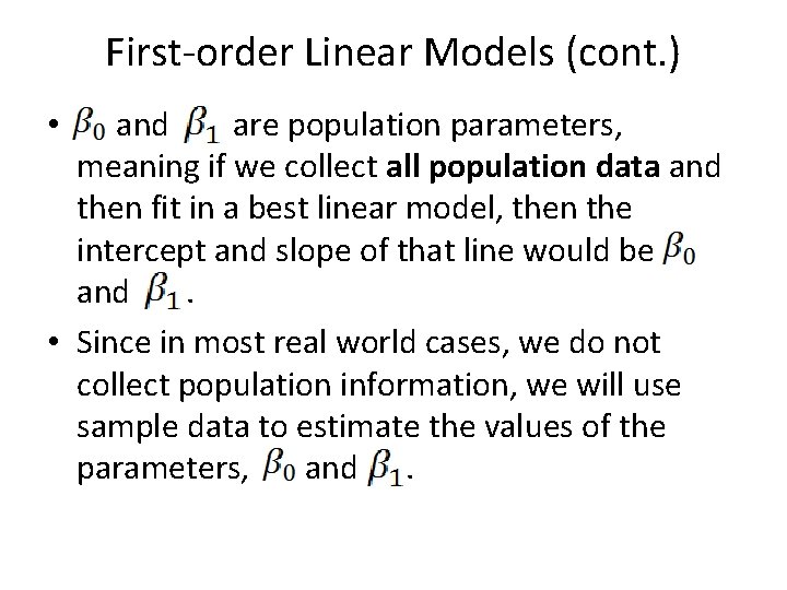
First-order Linear Models (cont. ) and are population parameters, meaning if we collect all population data and then fit in a best linear model, then the intercept and slope of that line would be and. • Since in most real world cases, we do not collect population information, we will use sample data to estimate the values of the parameters, and. •

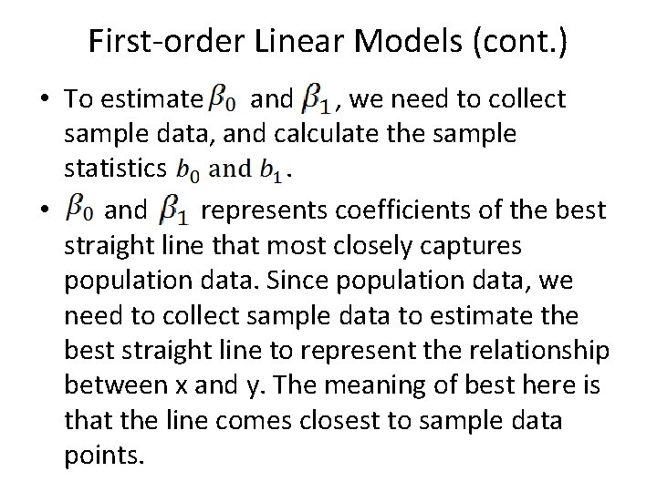
First-order Linear Models (cont. ) • To estimate and , we need to collect sample data, and calculate the sample statistics. • and represents coefficients of the best straight line that most closely captures population data. Since population data, we need to collect sample data to estimate the best straight line to represent the relationship between x and y. The meaning of best here is that the line comes closest to sample data points.

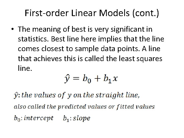
First-order Linear Models (cont. ) • The meaning of best is very significant in statistics. Best line here implies that the line comes closest to sample data points. A line that achieves this is called the least squares line.

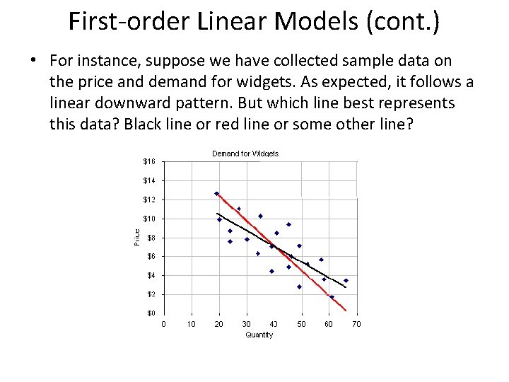
First-order Linear Models (cont. ) • For instance, suppose we have collected sample data on the price and demand for widgets. As expected, it follows a linear downward pattern. But which line best represents this data? Black line or red line or some other line?

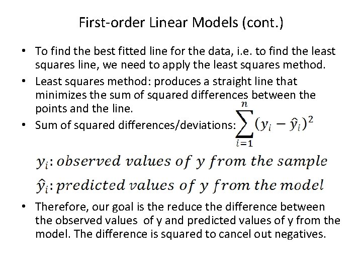
First-order Linear Models (cont. ) • To find the best fitted line for the data, i. e. to find the least squares line, we need to apply the least squares method. • Least squares method: produces a straight line that minimizes the sum of squared differences between the points and the line. • Sum of squared differences/deviations: • Therefore, our goal is the reduce the difference between the observed values of y and predicted values of y from the model. The difference is squared to cancel out negatives.

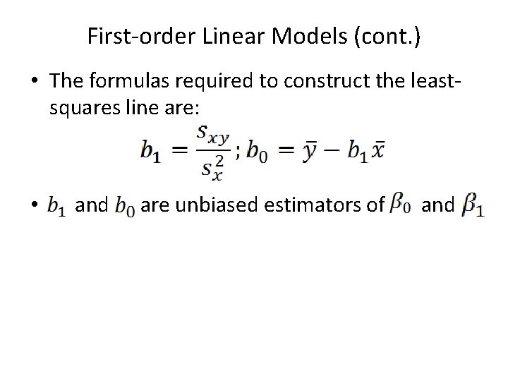
First-order Linear Models (cont. ) • The formulas required to construct the leastsquares line are: • and are unbiased estimators of and

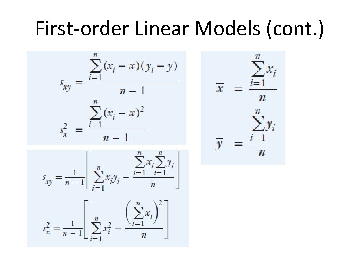
First-order Linear Models (cont. )

Example 1

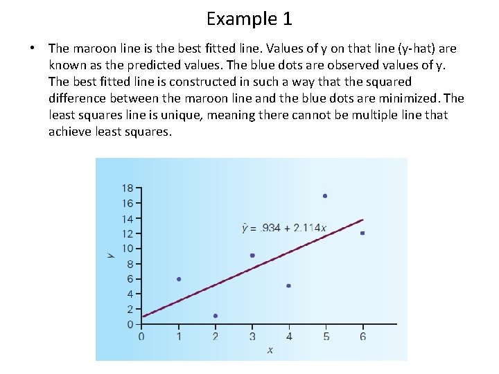
Example 1 • The maroon line is the best fitted line. Values of y on that line (y-hat) are known as the predicted values. The blue dots are observed values of y. The best fitted line is constructed in such a way that the squared difference between the maroon line and the blue dots are minimized. The least squares line is unique, meaning there cannot be multiple line that achieve least squares.

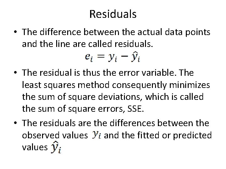
Residuals • The difference between the actual data points and the line are called residuals. • The residual is thus the error variable. The least squares method consequently minimizes the sum of square deviations, which is called the sum of square errors, SSE. • The residuals are the differences between the observed values and the fitted or predicted values

Residuals (cont. )

Residuals (cont. )

Residuals (cont. ) • Since we have used least squares method, no other straight line will produce a sum of squared deviations as small as 81. 04. This means that the regression line fits the data best.

Example 2

Example 2 Interpretations